Research Discussion Paper – RDP 2021-07 Macroprudential Limits on Mortgage Products: The Australian Experience
1. Introduction
Twice between 2014 and 2018, the Australian Prudential Regulation Authority (APRA) temporarily restricted banks' lending in mortgage types considered systemically risky. The first policy, announced late 2014, required banks to limit their lending to housing investors, or in other words, ‘buy-to-let’ borrowers that will rent out the housing. The second policy, announced early 2017, imposed limits on interest-only (IO) mortgages, in which the loan principal stays constant and only interest is repaid. APRA (2019b) describes the policies as ‘tactical, temporary constraints’, because they were designed to act fast and target the specific sources of systemic risk. Credit was expanding rapidly in residential mortgage products considered procyclical, while housing prices and household debt were high and rising (Debelle 2018; APRA 2019b). The limits were later removed, replaced by longer-term solutions.[1]
Macroprudential credit growth limits are backed by a deep literature tying credit growth to financial crises. Research shows that excessive credit growth is the most consistent antecedent of financial crises (e.g. Borio and Lowe 2002; Reinhart and Rogoff 2011; Schularick and Taylor 2012). Speculative mortgage debt and housing price cyclicality were fundamental ingredients in the 2008 financial crisis (Adelino, Schoar and Severino 2016; Foote, Loewenstein and Willen 2021), and contributed to crises further back (Dell'Ariccia et al 2012; Richter, Schularick and Wachtel 2021). The evidence has led to policy action. A variety of macroprudential tools have been implemented to curb excessive or risky credit (e.g. Cerutti, Claessens and Laeven 2017), including many specifically targeting mortgage lending (e.g. Kuttner and Shim 2016).
To our knowledge, none of these policies have targeted overall growth in particular mortgage products, aside from APRA's.[2] APRA's first policy required each bank to limit its year-ended growth in investor housing credit to 10 per cent. The second policy required each bank to limit its quarterly new IO mortgage lending to 30 per cent of total new housing lending. Most policies in other countries have set quantitative requirements only on loans above specific loan-to-valuation ratios (LVRs) or loan-to-income ratios (LTIs). APRA did present guidance that banks should manage new lending at high LVRs and LTIs, but quantitative limits were only set for the specific mortgage products. This was for a few reasons: high LVR lending was already in decline, limits on high LVR loans can disproportionately affect first home buyers, and the main risks appeared concentrated in speculative and IO borrowing (Ellis and Littrell 2017; APRA 2019b).
Our paper presents a bank-level panel data study of banks' reactions to the policies. We present causal statistical evidence, with falsification tests, that the policies reduced growth in the policy-targeted mortgage products. Banks cut lending growth in targeted mortgages by around 20 to 40 percentage points within a year of the policy announcements. While conclusions about systemic stability are outside this paper's scope, the findings are consistent with the policies achieving their objectives. We also present 3 conclusions, which build on existing qualitative analysis of the policies by the Australian Competition and Consumer Commission (ACCC), APRA and the Australian Government Productivity Commission (PC):
- Banks cut back targeted mortgage types by raising interest rates on those mortgages. This has been noted by, for example, ACCC (2018a, 2018b). We contribute by presenting causal statistical evidence, which estimates policy-induced rises in advertised rates of around 10 to 30 basis points, and by tying together banks' quantity and price responses. These rate rises partly reflected a desired repricing of risk, although ACCC (2018a, 2018b) also argue that the policies presented a focal point for coordinated anti-competitive price changes. We find that banks' mortgage interest income rose after the IO policy, in line with the ACCC's conclusion, but that the effect was short-lived.
- Banks' policy reactions depended on their size. Large banks – that is, the 4 Australian major banks – substituted into non-targeted mortgage types, and sustained their overall mortgage growth. The 20 or so other (mid-sized) banks in our sample did not substitute and their overall mortgage growth declined. These bank-level patterns are statistically significant but, in aggregate, coincide with only a small temporary pick-up in large banks' mortgage market share relative to the other sample banks. To our knowledge we are the first to show that banks' credit allocation reactions to macroprudential policies depend on their size.
- Implementation difficulties significantly influenced how the policies played out. Banks reacted to the investor policy with a 2-quarter delay, and their reaction sizes were misaligned with the policy impositions. These results support conclusions in previous regulatory reports that banks' systems initially lacked the capacity to control growth in the targeted mortgage types, and, for mid-sized banks, this imperfect control was compounded by heavy customer flows from the large banks' policy reactions. Contacts also tell us that some banks were uncertain about the precise definition and time frame for the investor limit, which contributed to the delayed reactions. Practical difficulties were less prevalent for the IO policy, after banks had improved their systems, and with the policy worded more precisely.
Our work presents several other results. Analysis of aggregate credit indicates that the policies had little effect on overall housing credit growth – with large banks substituting across housing credit types – and, if anything, a positive effect on business credit. Analysis of granular mortgage categories reveals that the accompanying guidance on high LVR lending, mentioned above, interacted with the quantitative limits: the decline in targeted housing credit was concentrated in high LVR loans, and substitution into non-targeted housing credit was concentrated in low LVR loans. We also argue that the substitutability between targeted and non-targeted mortgages differed across the 2 policies due to the types of products targeted. While a bank can steer any given customer towards either an IO or a principal and interest (P&I) loan, by offering attractive interest rates (e.g. Guiso et al forthcoming), customers typically cannot switch their status from investor to occupier. Therefore, to substitute from investor to occupier credit, banks need to find other customers, which Acharya et al (2020) call the ‘bank portfolio choice’ channel. This likely made substitution easier under the IO policy relative to the investor policy. More generally, across the full sample we find that IO and investor lending move with housing prices, while occupier P&I lending does not. This is consistent with speculative demand being driven by recently observed price behaviour.
This paper contributes to the growing literature studying the variety of macroprudential credit growth policies implemented around the world. In line with the other policies implemented, most papers focus on the impact of LTI and LVR limits. Results typically show a reduction in the targeted mortgages, particularly by banks exceeding specified limits. Some find that banks under the limits lift mortgage originations, in targeted mortgages (in the United Kingdom, Peydró et al (2020)), or in non-targeted mortgages (in Ireland, Acharya et al (2020)). We find that substitution into non-targeted mortgages is mostly by banks above the limits, which in our sample tend to be the largest banks, with potentially more capability to shift their portfolios. Many studies also find a significant negative effect on housing prices, including in the United Kingdom (Peydró et al 2020), in New Zealand (Armstrong, Skilling and Fao 2019) and in cross-country studies (Kuttner and Shim 2016; Alam et al 2019; Araujo et al 2020). We do not analyse housing price effects, but note that RBA (2018) finds that the investor policy caused housing price growth to slow more in investor-concentrated regions than in occupier-concentrated regions. More broadly, ours and these other papers on credit growth limits contribute to the wider literature on macroprudential policy effects (e.g. Aiyar, Calomiris and Wieladek 2014; Cerutti et al 2017; Jiménez et al 2017).
Banks' use of interest rates to target credit growth has been less studied. Basten (2020) shows that, following the introduction of the countercyclical capital buffer (CCyB) in Switzerland, capital-constrained banks raise their mortgage rates more than others. DeFusco, Johnson and Mondragon (2020) show that US lenders charge a premium of 10 to 15 basis points to originate loans above a regulatory debt-to-income ratio threshold (under the Dodd Frank Act), above which mortgages require extra ‘ability to repay’ documentation. We find interest rate policy effects of a similar magnitude. They also find that banks additionally contained quantities through credit rationing, which led to irregular demand elasticities, and we also find that banks limited credit supply through means other than rate rises.
The rest of this paper is laid out as follows. We first describe the investor and IO policies (Section 2). As background for the analytical results, the next sections explain the dataset and the variables of interest (Section 3) and the econometric models we use (Section 4). Then we report results for policy effects on banks' credit growth and interest rates, first for the investor policy (Section 5), and then for the IO policy (Section 6). Section 7 presents findings for other outcomes of interest: banks' LVR distributions (7.1); aggregate credit trends (7.2.1); banks' housing credit market shares (7.2.2); banks' mortgage pricing power (7.2.3); borrowers' reclassifications of mortgage types (7.3); and, more generally, the cyclicality of mortgage behaviour throughout the sample (7.4). Section 8 concludes.
2. The Credit Growth Limits
APRA's 2 macroprudential policies were announced in late 2014 and early 2017, respectively. The policy designs had 4 goals: efficient and well-targeted on the identified risks; competitively neutral across the industry, but with flexibility for smaller banks; able to be implemented quickly and simply; and able to be dialled up or down as required (APRA 2019b). The 2 quantitative limits were the most significant components of a package of measures that more broadly increased the intensity of housing lending oversight. The overarching objectives of this package were to strengthen the resilience of individual ADIs, and to promote the stability of the financial system overall.[3]
The policies were supported by the Council of Financial Regulators, which comprises APRA, the Australian Securities and Investments Commission, the Reserve Bank of Australia (RBA), and the Australian Treasury. The risk environment that led to the policies is described in most detail by RBA (2018). The main concern was that the targeted mortgage types were contributing to a housing market upswing that raised the risk of a subsequent economic downturn. Alongside rapidly rising investor housing credit, housing prices were rising and household debt was growing at its fastest pace in around a decade. This presented the risk that if income or housing prices subsequently fell, highly indebted households might react with a sharp reduction in consumption.
The rest of this section provides more details on the 2 quantitative limits.
2.1 The investor mortgage limit
APRA announced the investor limit on 9 December 2014 through a public letter to ADIs. Letters to ADIs do not constitute binding prudential requirements, but can present information about how APRA will exercise discretionary regulatory powers. The letter states that:
… annual investor [housing] credit growth materially above a benchmark of 10 per cent will be an important risk indicator that supervisors will take into account when reviewing ADIs' residential mortgage risk profile and considering supervisory actions. (APRA 2014)
In the following months, the expectations that banks comply with the limit were ramped up. APRA (2019b, p 13) writes that:
… over the first half of 2015, APRA supervisors took coordinated action to reinforce the objectives of the benchmark with all ADIs and obtain action plans for meeting it … In a number of cases, supervisors agreed on an appropriate timeline for meeting the expectations with individual ADIs …
By August, the 4 largest banks had each indicated to the RBA that they were then treating the benchmark as a hard limit.[4] The policy remained less strict for small banks with mortgage portfolios of less than $1 billion, which were given a longer horizon to comply.[5]
The letter to banks also stated that APRA would monitor other types of banks' lending. The other types included high LVR and high LTI mortgages, IO mortgages, mortgages with very long terms, and mortgages that did not perform well on borrower affordability tests. However, no quantitative requirements were stated for those mortgage types, then or later. We focus on the effects of the quantitative limits, but also analyse policy effects by LVRs in Section 7.1.
APRA removed the investor limit in April 2018, conditional on banks' boards providing assurance of ongoing safe lending practices. The limit was removed due to the actions banks had taken to improve the quality of their lending (APRA 2019b). It was replaced with longer-term tools for distinguishing between mortgage products in their systemic risk contributions. In February 2018, APRA released proposed changes to ADIs' capital framework that would impose higher risk weights for investor mortgages than occupier mortgages, and reaffirmed its proposal in December 2020. Additionally, in July 2019, APRA released a revised Prudential Practice Guide that outlined APRA's interpretation of prudent practices in residential mortgage lending (APRA 2019a), to supplement APRA's legally enforceable Prudential Standards.
2.2 The interest-only mortgage limit
APRA announced the IO limit on 31 March 2017 in another letter to ADIs. The letter asked banks to limit new IO lending to no more than 30 per cent of total new mortgage lending. From the start, the expectations were stricter than for the investor policy. The letter states ‘APRA supervisors … will likely impose additional requirements on an ADI if the proportion of new lending on interest-only terms exceeds 30 per cent of total new mortgage lending, over the course of each quarterly period’, and ‘APRA expects all ADIs to immediately take steps’ (APRA 2017). IO mortgages were a concern in part because the lack of amortisation keeps the borrower's leverage higher for longer, and in part because IO mortgages automatically convert to P&I loans, usually after 5 to 10 years, which can, if the mortgage is not refinanced to another IO loan, bump up the repayments and can cause distress for the borrower (Kent 2018).
APRA also noted it would monitor other metrics of risk in banks' new mortgage lending, in a similar manner to the guidance accompanying the investor limit. Again, there were no quantitative requirements on those metrics. In December 2018, APRA removed the limit, stating that the policy had served its purpose.
3. Data and Variables
This section details the data, sample and variables used for the empirical analysis. Section 3.1 describes the data sources and the sample choices. Section 3.2 defines the regression variables and provides summary statistics.
3.1 Datasets and sample
The two main data sources comprise banks' confidential data reporting to APRA, and banks' advertised mortgage rates from the subscription-based Canstar database. We supplement these with housing price data from the subscription-based CoreLogic database and publicly available national accounts data from the Australian Bureau of Statistics (ABS).
The sample is quarterly, from 2008:Q1 to 2019:Q3, and covers banks with at least $1 billion in total loan assets. The regression samples each exclude banks that were not in the sample one year prior to the policy announcement, leaving around 28 banks in most cases. Sample banks are classified as either large or mid-sized. The large banks comprise the 4 major banks – ANZ, CBA, NAB and Westpac – which are each similar sized, and together hold around 80 per cent of total mortgage credit in Australia. The remaining banks are much smaller and classified as mid-sized. There were 3 mergers between sample banks during the sample period, so for the quarters prior to the merger, we combine the 2 pre-merged banks into 1 consolidated entity.
To analyse new housing lending, we use data on mortgage commitments. A mortgage commitment takes place after the borrower receives an accepted and signed offer of credit from the lender, typically after the borrower has signed the contract for purchase of the property.[6] Commitments are categorised by either the borrower type (occupier or investor), or by the repayment structure (P&I or IO), or by both. Commitments are a better measure of mortgage origination than changes in credit outstanding, for 2 reasons. First, following the policy announcement in December 2014, banks raised interest rates on investor mortgages (Section 5.2), and many customers updated their bank about their classification as an investor or occupier. This heavily affected credit quantities outstanding, despite not generating mortgage originations, but only rarely would have affected commitments. These reclassifications are discussed further in Section 7.3. Second, credit outstanding can move for reasons unrelated to new lending, such as refinancing, early repayments, or drawing down on excess balances. Nonetheless, commitments do not perfectly map to new mortgage lending (i.e. originations), which was the target of the limits. Commitments typically lead originations by a few weeks, and in some cases result in no origination.
The Canstar data on advertised mortgage rates cover various mortgage subtypes and require some discretionary alignment with the 4 categories of approvals (occupier P&I, occupier IO, investor P&I, investor IO).[7] It is important to note that the advertised rates do not cleanly represent rates charged. Borrowers often receive a discount on the advertised rate, which is more common among large banks than mid-sized banks. Our analysis of advertised rates could therefore miss policy effects on discounts, which did occur to some extent (e.g. ACCC 2018b). However, when analysing targeted mortgages, this would more likely understate than overstate the policy effect estimates. That is, given that banks were using rates to reduce demand for targeted mortgages (Sections 5.2 and 6.2), discounts were more likely to be lowered rather than raised, in which case the rises in advertised rates would understate the rises in offered rates. For non-targeted mortgages, the opposite holds true, so it is possible that those estimates of policy effects on interest rates are overstated, particularly for large banks.
3.2 Regression variables
The 2 main dependent variables are commitments growth and mortgage rates . measures the percentage change in the total dollar value of mortgage commitments from quarter t–1 to quarter t, for mortgage type m {investor, occupier, IO, P&I, Total} and by bank b. It is expressed as a decimal, so, for example, 10 per cent growth is 0.1. All infinite values are excluded (i.e. when a bank grows commitments from zero) and remaining outliers above 300 per cent are truncated to 3.
The dependent variable measures bank b ′s advertised mortgage rate at the end of quarter t, minus the cash rate, in percentage points. It is first differenced in most regressions. When analysing the investor policy, ‘investor rates’ are from investor P&I mortgages, and ‘occupier rates’ are from occupier P&I mortgages. When analysing the IO policy, ‘IO rates’ are from investor IO mortgages and ‘P&I rates’ are from investor P&I mortgages. This approach varies the mortgage-type dimension affected by the policy while holding the other dimension constant. It also avoids relying on rates for occupier IO mortgages, which are less common than other mortgage types.
The 2 key explanatory variables are a bank-invariant indicator variable for the quarter a policy is announced (𝕀(policy)t) and a measure of how far bank b is from the policy limit ( Treatmentb,t ). 𝕀(policy)t is one in the quarter t the policy is announced, and zero in other quarters. Most regressions use its first to fourth lags, which capture policy effects in the 4 quarters after the announcement. Treatmentb,t takes 2 alternative forms: linear and binary. For the investor policy, the linear measure is the bank's year-ended growth in the total value of investor mortgages outstanding, minus 10 per cent, measured in percentage points.[8] For the IO policy, the linear measure is the proportion of the bank's quarterly housing commitments that are IO commitments, minus 30 per cent, measured in percentage points. As noted in Section 3.1, the policy referred to the proportion of new mortgage lending, but we do not have data on originations, so we use commitments as a close proxy. The binary form of Treatmentb,t is an indicator variable for whether bank b is above the limit in quarter t, or in other words, for whether the linear form of Treatmentb,t is positive.
The regressions also include sets of macroeconomic and bank-level control variables. The (bank invariant) macroeconomic controls include quarterly growth in national GDP (from the ABS), quarterly growth in national housing prices (from CoreLogic), and the first difference in the quarter-end ‘cash rate’, which is Australia's key monetary policy rate (from the RBA).[9] These are all expressed in percentages. The macroeconomic controls also include a set of seasonal indicator variables that control for the 4 quarters each year – for example, a ‘Q2’ indicator, which is 1 in Q2 each year and 0 in other quarters – because commitments tend to be highly seasonal (evident in Figure 1 below). In the regression formulas, the vector of macroeconomic controls is represented by MacroControlst. The bank-level controls are the tier 1 capital ratio and the ratio of deposit liabilities over total liabilities, both expressed in percentage points, sourced from the confidential APRA data. These are represented in the regression formulas by BankControlsb,t.
The regression variables are summarised in Table 1. Most of the regression samples separate large from mid-sized banks. The size difference between large and mid-sized banks is clear from the commitments values. Large banks' mean value of quarterly total commitments is $14.8 billion, with a $4.5 billion standard deviation, while mid-sized banks' mean is $0.9 billion and standard deviation is also $0.9 billion. Commitments growth rates are similar for large and mid-sized banks, but vary more across mortgage types for mid-sized banks. Large banks tend to advertise higher spreads than mid-sized banks, but this likely reflects that large banks more commonly offer discounts off the advertised rate. (The regressions mostly analyse changes in spreads, so any time-invariant influence of discounting would be removed.) Mid-sized banks rely on deposit funding more so than large banks.
| Large banks | Mid-sized banks | Full sample | ||||||||||
|---|---|---|---|---|---|---|---|---|---|---|---|---|
| Mean | SD | Mean | SD | Min | 25% | Median | 75% | Max | Number | |||
| Mortgage commitments quarterly value ($b) | ||||||||||||
| Investor | 5.2 | 2.2 | 0.3 | 0.3 | 0.0 | 0.1 | 0.2 | 0.8 | 11.3 | 946 | ||
| Occupier | 9.6 | 2.8 | 0.6 | 0.6 | 0.0 | 0.2 | 0.6 | 1.8 | 17.1 | 946 | ||
| Interest only (IO) | 5.0 | 2.7 | 0.2 | 0.3 | 0.0 | 0.0 | 0.2 | 0.8 | 12.7 | 946 | ||
| Principal and interest (P&I) | 9.8 | 3.8 | 0.7 | 0.7 | 0.0 | 0.2 | 0.6 | 1.9 | 20.0 | 946 | ||
| Total | 14.8 | 4.5 | 0.9 | 0.9 | 0.0 | 0.3 | 0.8 | 2.6 | 26.3 | 946 | ||
| Mortgage commitments quarterly growth (%) | ||||||||||||
| Investor | 8.4 | 46.8 | 11.0 | 49.5 | −100.0 | −13.5 | 2.6 | 22.5 | 300.0 | 918 | ||
| Occupier | 8.1 | 45.6 | 6.7 | 34.9 | −94.6 | −10.7 | 2.2 | 16.4 | 300.0 | 919 | ||
| IO | 7.5 | 48.6 | 10.9 | 55.7 | −100.0 | −16.8 | 0.7 | 24.2 | 300.0 | 916 | ||
| P&I | 8.6 | 45.5 | 7.4 | 37.1 | −94.8 | −10.5 | 2.2 | 17.0 | 300.0 | 919 | ||
| Total | 8.0 | 45.6 | 6.5 | 34.4 | −95.5 | −10.4 | 1.6 | 16.1 | 300.0 | 919 | ||
| Change in mortgage rate spread to cash rate (to quarter-end, bps) | ||||||||||||
| Investor P&I | 4.4 | 10.2 | 2.1 | 20.5 | −238.0 | 0.0 | 0.0 | 5.5 | 80.0 | 1,133 | ||
| Occupier P&I | 3.0 | 11.9 | 1.3 | 17.6 | −162.0 | 0.0 | 0.0 | 2.0 | 75.0 | 1,183 | ||
| P&I investor–occupier spread | 1.5 | 12.9 | 0.7 | 14.0 | −80.0 | 0.0 | 0.0 | 0.0 | 89.0 | 1,130 | ||
| Investor IO | 5.3 | 12.5 | 2.5 | 22.5 | −246.0 | 0.0 | 0.0 | 9.0 | 80.0 | 944 | ||
| Investor IO–P&I spread | 0.9 | 8.6 | 0.1 | 11.9 | −136.0 | 0.0 | 0.0 | 0.0 | 157.0 | 929 | ||
| Bank-level control variables (%) | ||||||||||||
| Tier 1 capital ratio | 11.1 | 1.5 | 13.7 | 4.6 | 6.5 | 10.4 | 12.2 | 15.1 | 32.5 | 984 | ||
| Deposit over liabilities ratio | 47.8 | 7.3 | 71.0 | 21.2 | 11.8 | 46.9 | 67.8 | 86.4 | 99.0 | 984 | ||
|
Sources: APRA; Authors' calculations; Canstar; RBA |
||||||||||||
Figure 1 displays the aggregate behaviour of some key variables. Most commitments are for occupier P&I mortgages, with the remaining commitments roughly equally split across the other 3 mortgage types, until around 2013 when investor IO commitments pick up (top panel). Commitments have clear seasonality in a 4-quarter cycle. Average mortgage rates across banks are initially very close for different mortgage types, until after the first policy announcement in late 2014 (middle panel). Comparing the middle and bottom panels makes clear that mortgage rates move fairly closely with the cash rate. The most noteworthy behaviour in the macroeconomic variables is in 2015, when the investor policy was being implemented (bottom panel). In the first half of 2015, the cash rate is cut twice – by 25 basis points in both February and May – but it remained constant for the rest of 2015, and throughout 2017 and 2018. Also in the second half of 2015, housing price growth declined from around 5 per cent per quarter to around zero. This is discussed briefly in Section 5.4.2.
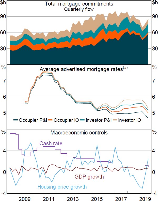
Note: (a) Mortgage rates as used in regressions, after cleaning and alignment; unweighted average across banks
Sources: ABS; APRA; Canstar; CoreLogic; RBA
4. Empirical Strategy
We identify policy effects with 2 types of panel data regressions. The first detects the average policy effect across all banks in the sample that is used. We supplement these estimates with falsification (i.e. placebo) tests that gauge the likelihood of falsely identifying policy effects. The second type detects policy effects that systematically differ across banks. The second type has a more robust identification strategy, so it provides a more definitive test of whether the policies caused a change in banks' behaviour. However, aggregate policy effects are less clear with this specification, hence the use of 2 separate strategies. Note that none of the specifications give more weight to banks with larger portfolios, so the outcomes should not be interpreted as aggregated effects on the banking system. (But that interpretation would be close for samples containing only the 4 large banks.) To understand aggregated effects we report aggregate time series throughout various parts of the paper.
4.1 Average effect regressions
The average effect regressions estimate the policy effects using (bank invariant) indicator variables for the 4 quarters after the policy announcement (𝕀(policy )t–1,…, t–4 ). Control variables remove other influences, leaving the indicator variables to capture any ‘abnormal behaviour’ in the policy period that is common across all banks in the sample. The controls include lagged dependent variables, other bank-level control variables, and system-level macroeconomic control variables.
The average effect regression equation is
In Equation (1), the lagged dependent variables are instrumented using the Arellano–Bond procedure. This involves first differencing all variables (as per Equation (1)). Bank fixed effects are therefore not included. The macro controls are GDP growth, housing price growth and the set of seasonal controls.[10] The bank controls are the capital ratio and the deposit funding ratio, both lagged once to address reverse causality.
The average effect specification for mortgage interest rates is
where is a set of bank-level fixed effects. The bank and macro controls are the same as in Equation (1), except the first 2 lags of the quarter-end change in the cash rate are added as macro controls, given that the cash rate is a very strong determinant of mortgage rates. Lagged dependent variables are included in Equation (1) but not in Equation (2), because mortgage rate changes are much less persistent than commitments growth.
The average effect regressions are repeated for mortgage types m not targeted by the policies. These non-targeted mortgages serve as a quasi control group. For example, if a decline in credit that is detected by 𝕀(policy) is instead spuriously driven by macroeconomic influences, this should be revealed by a negative policy effect in the non-targeted loan types. It is not appropriate to use non-targeted mortgages as an explicit control group in a differences-in-differences specification. This would lead to overstated policy effect estimates if banks substituted from targeted to non-targeted mortgages. However, we are still interested in the effects of the policy on non-targeted mortgages. So we examine them in separate estimations, but without including them as explicit controls in the same equation.
The main threat to identification is the possibility of system-wide influences that coincidentally affect (only) targeted mortgages when the policies are implemented, and that are not captured by the control variables. We address this in 2 ways. First, we run placebo regressions akin to the falsification tests suggested by Roberts and Whited (2013). In the placebo regressions, the 4 𝕀(policy) variables are swapped for a ‘placebo’ indicator variable that instead indicates a single non-policy quarter, to assess whether a false positive effect shows up in that quarter. This is repeated for all non-policy quarters from 2010 onward. If few of these placebo indicators are significant, the likelihood of coincidental factors causing a falsely detected policy effect is low. Due to the multiple testing problem (e.g. Bender and Lange 2001), these placebo tests warrant conservative significance thresholds, which we acknowledge informally. We also address the coincidental-influences identification threat with a qualitative analysis of economic trends that could have potentially generated false policy effects.
The average effect regressions are each run on multiple samples. One sample comprises only the 4 large banks, another sample comprises only mid-sized banks and a third sample comprises all banks.
4.2 Heterogeneous effect regressions
The heterogeneous effect regressions identify policy effects that differ across banks, in line with how close those banks are to satisfying the policy limits. Intuitively, banks above the limit should be more intensely ‘treated’ by the policy than banks below. Focusing on these differences in reactions across banks allows including fixed effects for each quarter, which in the average effect regressions would be collinear with 𝕀(policy). Quarter fixed effects remove all system-wide influences on the dependent variables, and give a stronger case for identification of the policy effects.
The heterogeneous policy effects regression equation is
Y is either CommitGrth or IntRate, and Treatment is a measure of how far bank b is above the limit. Treatment is lagged twice to remove reverse causality from mechanical dependence on commitments growth.[11] That is, distance from the limit in a given period likely depends on commitments in that period, and therefore on commitments growth in the next period (because growth rates depend on the level in the last period). Bank and quarter fixed effects are represented by and . The bank controls are the capital ratio and deposit funding ratio.
5. Policy Effects of the Investor Limit
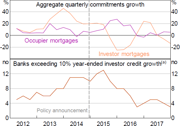
The investor mortgage limit, announced in December 2014, limited banks' growth in investor housing credit to 10 per cent per annum. Other regulatory reports document that the limit took time to implement (e.g. APRA 2019b), as APRA worked with banks to clarify their obligations (as noted in Section 2.1) and banks worked on improving their systems for implementing the policy. Contacts tell us that banks also initially faced some confusion over the definition of the limit, for example, about how to treat pre-existing investor credit that was being reclassified as occupier credit (analysed in Section 7.3), or whether the limit applied to raw or seasonally adjusted credit growth figures. A delay between the policy announcement and its effect is indeed evident in the aggregate data (Figure 2). Aggregate investor commitments growth remains flat in 2015:Q1 and Q2, then declines sharply in 2015:Q3 and Q4 alongside a pick-up in occupier commitments growth (top panel). The number of banks above the limit picks up in 2015:Q1 and Q2, but, from 2015:Q3 onward, steadily declines towards zero (bottom panel).
Notes:
The number of banks in the sample varies slightly across periods but is constant from 2014:Q3 to 2017:Q4
(a) May not perfectly align with APRA's assessment of banks meeting the limit
Sources: APRA; Authors' calculations
5.1 Average effects on mortgage commitments
In the full sample of banks, the policy effect on targeted mortgages is negative, large and statistically significant in 2015:Q3 and Q4 (Table 2, column (a)). The coefficients imply a decline in investor commitments growth of 51 percentage points across these 2 quarters, for the average bank.[12] There are no significant policy effects in the first 2 quarters, in line with the aggregate data (Figure 2), implying a 2-quarter delay from the policy announcement on average. Non-targeted mortgages increase by a statistically insignificant and small amount (column (b)), which implies that the estimated investor policy effects in column (a) are not mistakenly picking up trends in aggregate housing credit. Total mortgage commitments for the average bank are not significantly affected (column (c)). Therefore, the large reduction in investor commitments growth is mostly offset by the small pick-up in occupier commitments growth.
| Sample banks: |
(a) | (b) | (c) | (d) | (e) | (f) | (g) | (h) | (i) | ||
|---|---|---|---|---|---|---|---|---|---|---|---|
| All | Large | Mid-sized | |||||||||
| Mortgage type: | Investor | Occupier | Total | Investor | Occupier | Total | Investor | Occupier | Total | ||
| 𝕀(Q1–15) | –0.058 (0.052) |
0.024 (0.039) |
0.015 (0.039) |
−0.025** (0.011) |
−0.008 (0.011) |
−0.008 (0.007) |
−0.070 (0.062) |
0.029 (0.047) |
0.019 (0.047) |
||
| 𝕀(Q2–15) | −0.051 (0.070) |
0.005 (0.056) |
−0.013 (0.056) |
−0.059 (0.072) |
0.020 (0.071) |
0.003 (0.072) |
−0.031 (0.085) |
0.002 (0.067) |
−0.010 (0.066) |
||
| 𝕀(Q3–15) | −0.235*** (0.072) |
0.029 (0.054) |
−0.061 (0.049) |
−0.236*** (0.032) |
0.144* (0.086) |
−0.025 (0.051) |
−0.241*** (0.089) |
−0.005 (0.060) |
−0.072 (0.057) |
||
| 𝕀(Q4–15) | −0.337*** (0.094) |
0.024 (0.057) |
−0.080 (0.049) |
−0.025 (0.051) |
0.096** (0.044) |
0.055 (0.036) |
−0.423*** (0.108) |
0.002 (0.069) |
−0.116** (0.057) |
||
| Lagged DVs | 2 | 2 | 2 | 2 | 2 | 2 | 2 | 2 | 2 | ||
| Controls | yes | yes | yes | yes | yes | yes | yes | yes | yes | ||
| Sample size | 686 | 686 | 686 | 168 | 168 | 168 | 518 | 518 | 518 | ||
| Notes: Coefficients from panel regressions, across banks and quarters, of commitments growth on 4 lags of the bank-invariant policy indicator variable. The full equation is in first differences, using Arellano–Bond, with 2 lagged dependent variables (DVs) to eliminate second order autocorrelation. The control variables are GDP growth, housing price growth, lagged tier 1 capital ratios, lagged deposit funding ratios and a set of seasonal dummy variables. ***, ** and * denote statistical significance at the 1, 5 and 10 per cent levels, respectively. | |||||||||||
The full sample estimates mask sizeable differences in reactions between large and mid-sized banks. Most notably, large banks substitute into non-targeted mortgages while mid-sized banks do not. Large banks' substitution into occupier commitments (column (e)) offsets their investor commitments growth decline, leaving no significant change in total mortgage commitments (column (f)). Mid-sized banks do not increase occupier commitments growth (column (h)), leaving a statistically significant net decline in total commitments growth of 12 percentage points (column (i)). The reason for this difference in substitution behaviour is not entirely clear, but it is plausible that large banks' operational systems were more capable of implementing a portfolio shift. The full sample estimates for occupier and total commitments show little policy effect (columns (b) and (c)) because large banks' expansions and mid-sized banks' contractions are netted against each other.
Large banks' substitution from investor to occupier credit is consistent with the ‘portfolio choice channel’ theory by Acharya et al (2020). The theory posits that, in general, banks leave some credit demand unmet because they face balance sheet constraints on their credit supply, such as regulatory capital and liquidity requirements. This leaves banks with capability to shift their credit portfolios toward a different customer segment, because potential customers with unmet demand are always available in that segment. Another possible explanation for the substitution is that the reduction in investor credit ‘made room’ for a pick-up in occupier demand. This could occur if a decline in investor activity caused lower housing price growth, which in turn expanded the number of occupiers that could afford to buy. Indeed, housing price growth declined in 2015:Q3 and Q4 – see Figure 1 and Section 5.4.2.
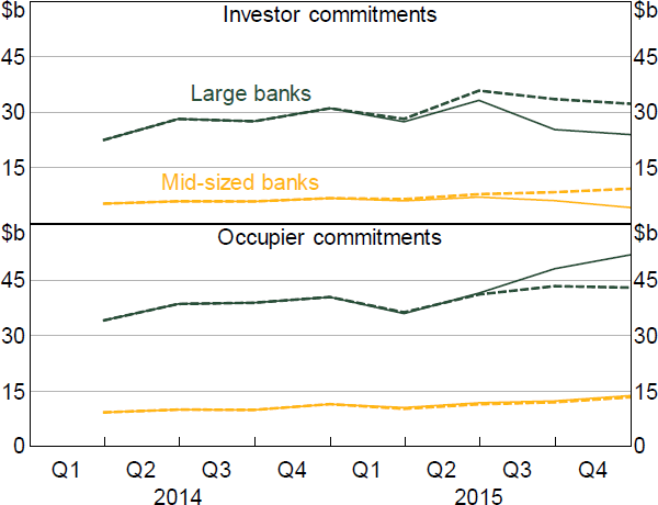
To contextualise the estimated effects, we plot observed total commitments against counterfactual estimates of what would have occurred without the policy (Figure 3), constructed using the coefficients in Table 2.[13] In the quarters before the policy, observed investor commitments steadily rise, fluctuating with seasonal patterns. The policy effects are then visible in the observed series, which drops lower than usual in 2015:Q3 and Q4. The counterfactuals suggest commitments would have been relatively flat absent the policy. The plot also demonstrates the different Q4 outcomes for large and mid-sized banks. For large banks, the total Q4 pick-up in occupier commitments roughly offsets the decline in investor commitments (both around $4 billion), while for mid-sized banks, only investor commitments are affected.
Sources: APRA; Authors' calculations
5.2 Average effects on advertised interest rates
Banks lifted interest rates on investor mortgages in 2015:Q3 (Table 3), the same quarter that investor commitments declined (Section 5.1).[14] In this quarter, large and mid-sized banks raised the spread between investor and occupier mortgage rates by around 10 basis points, by increasing investor rates.[15] RBA (2018) notes that this was the first time that banks systematically price differentiated these products, which is consistent with the aggregate data in Figure 1. Other regulatory reports explain that, after the policy was announced, banks first tried meeting the policy limit by imposing internal limits on loan-application acceptances, and resorted to interest rate increases when the internal limits did not suffice (ACCC 2018a; APRA 2019b).
| Sample banks: |
(a) | (b) | (c) | (d) | (e) | (f) | |
|---|---|---|---|---|---|---|---|
| Large | Mid-sized | ||||||
| Dependent variable: | Investor | Occupier | Spread | Investor | Occupier | Spread | |
| 𝕀(Q1–15) | −0.085** (0.033) |
−0.044 (0.031) |
−0.041 (0.026) |
−0.095*** (0.023) |
−0.088*** (0.020) |
−0.008 (0.026) |
|
| 𝕀(Q2–15) | 0.022 (0.040) |
−0.030 (0.045) |
0.052* (0.028) |
−0.059* (0.034) |
−0.017 (0.019) |
−0.045* (0.026) |
|
| 𝕀(Q3–15) | 0.128*** (0.024) |
0.020 (0.025) |
0.107*** (0.017) |
0.134*** (0.024) |
0.042 (0.033) |
0.095*** (0.020) |
|
| 𝕀(Q4–15) | 0.112*** (0.024) |
0.122*** (0.026) |
−0.010 (0.017) |
0.089*** (0.016) |
0.030* (0.017) |
0.057*** (0.014) |
|
| Fixed effects | Bank | Bank | Bank | Bank | Bank | Bank | |
| Other controls | yes | yes | yes | yes | yes | yes | |
| R squared | 0.241 | 0.295 | 0.098 | 0.157 | 0.280 | 0.108 | |
| Sample | 164 | 164 | 164 | 648 | 666 | 647 | |
|
Notes: Coefficients from panel regressions, across banks and quarters, of change in advertised mortgage rates on 4 lags of the bank-invariant policy indicator variable. The control variables are GDP growth, housing price growth, lagged tier 1 capital ratios, lagged deposit funding ratios and a set of seasonal dummy variables. The regressions include bank fixed effects. Standard errors are clustered at the quarter level for the large bank regressions, and at the bank and quarter levels for the mid-sized bank regressions. ***, ** and * denote statistical significance at the 1, 5 and 10 per cent levels, respectively. |
|||||||
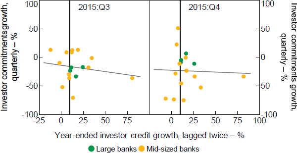
The rate increases are not neatly aligned with the reactions in commitments reported in Section 5.1. The policy-induced rate rises are supply-side driven, rather than caused by a change in credit demand, so we would expect a negative relationship between changes in interest rates and commitments growth. That is, the banks that raise rates most should experience the largest proportional reduction in customers. This holds true in aggregate – investor rates rise and investor commitments growth falls – but not across the cross-section. For example, in 2015:Q4, investor commitments growth falls heavily for mid-sized banks but not for large banks, despite large banks lifting investor rates by 2 basis points more.[16]
These irregular price–quantity relationships warrant further exploration. We hone in on 2015:Q3 and Q4, and plot each bank's investor commitments growth against its change in investor rates (Figure 4). We also acknowledge that commitments may not co-move tightly with rate changes over short periods, but that banks with consistently lower rates should experience more commitments growth over time. To achieve this, the plots show commitments growth from the level in 2015:Q2 to the average across the next 6 or 12 months (Figure 4, bottom panels). The rate changes are averaged the same way.
Bottom panels: from 2015:Q2 to (subsequent averages)
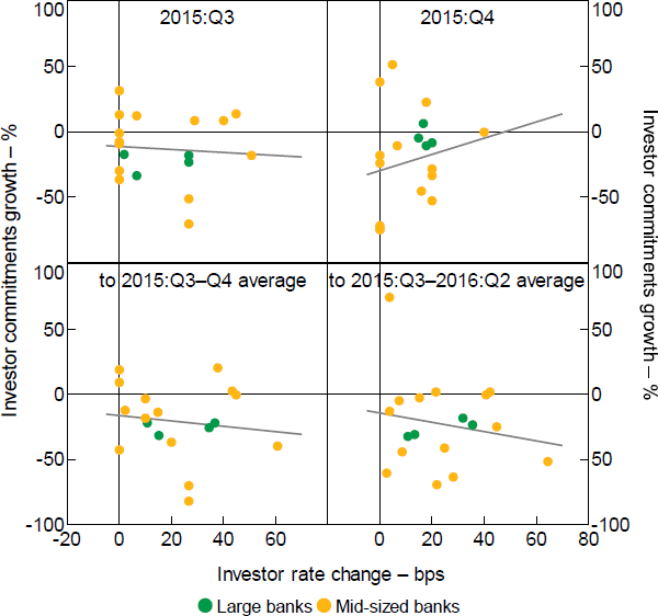
Notes: Rates are advertised rates, as described in Section 3.2; fitted lines are from OLS on plotted observations
Sources: APRA; Authors' calculations; Canstar
The plots indeed reveal counterintuitive price–quantity relationships across banks, but which become more intuitive at longer time horizons. In 2015:Q3, some mid-sized banks experience investor commitments growth of around –40 per cent without having lowered investor rates, and others experience positive growth after raising rates by around 40 to 50 bps. This is more extreme in Q4: some experience investor commitments growth of around –70 per cent without having lowered investor rates, and overall, banks with larger rate rises experience more commitments growth (i.e. the upward sloping fitted line in the top right panel). The erratic patterns in 2015:Q4 partly wash out at lower frequencies – the bottom panels of Figure 4 show a negative relationship between rates and commitments.
The counterintuitive relationships likely reflect a shake-up from the policy-induced credit reallocation. For mid-sized banks, the customer spillover from large banks shifting their far larger portfolios likely exceeded any typical fluctuations in demand. APRA (2019b, p 11) writes
… APRA did observe this spillover effect to some degree when the benchmarks were initially introduced. As it was, many smaller ADIs found themselves with an unanticipated surge in demand for credit that in some cases was difficult to manage. APRA sought to address concerns about impacts on smaller ADIs' ability to compete by adopting a more flexible approach to application of the benchmarks in the early stages …
Indeed, some banks reportedly reacted by temporarily stopping investor lending completely (PC 2018). We are told by contacts that these effects were also compounded by the role of mortgage brokers. That is, brokers would sometimes direct all their customers to the single bank with lowest rates, potentially a mid-sized bank that had been slower to raise its rates than other banks.
Our findings are consistent with these reports. For example, the reported spillover effects could explain why, in 2015:Q3, some mid-sized banks have positive commitments growth while lifting rates by around 30 to 50 basis points (Figure 4, top left panel). Further, the largest Q4 declines in investor commitments growth (Figure 4, top right panel) – which are not accompanied by rate rises – are consistent with some mid-sized banks temporarily stopping investor lending. Removing those observations would indeed leave a more intuitive negative relationship between prices and quantities. Furthermore, the role of mortgage brokers mentioned above would likely wash out at longer time horizons, as banks that are slower to move rates then catch up, and demand reacts accordingly. Consistent with this, the price–quantity relationships in Figure 4 are more negative for the longer time horizons (i.e. the bottom panels).
5.3 Heterogeneous effects
Specification (3) identifies the policy effect by estimating the difference in responses between banks above and below the limit. The results do not show a clear effect with either measure of policy treatment (Table 4). In the third and fourth quarters, investor commitments growth is indeed lower for banks further above the limit (the column (a) coefficients are negative). However, the effect is not statistically significant, and more broadly, the coefficient signs in columns (a) to (d) are not consistent with the expected heterogeneous effect (negative for investor commitments, positive for occupier commitments). Banks above the limit raise rates more than others in 2015:Q3 and Q4, but roughly equally for targeted and non-targeted mortgages (columns (e) to (h)). The results provide little indication that banks' responses to the policy depend on their distance from the limit (columns (a) to (c)) or whether they exceed the limit (columns (d) to (e)).
The lack of relationship between the policy treatment and changes in investor commitments growth is visualised in Figure 5. In Q3 and Q4, most banks above the limit indeed reduce their investor commitments growth, but this is also true for banks below the limit. This is consistent with the unpredictability of conditions facing mid-sized banks that is discussed in Section 5.2. Mid-sized banks below the limit, concerned about unpredictable flows pushing them above the limit, may have reduced investor commitments as a precaution, including by raising investor rates.
| Dependent variable: |
(a) | (b) | (c) | (d) | (e) | (f) | (g) | (h) | |||
|---|---|---|---|---|---|---|---|---|---|---|---|
| Commitments growth | Rate changes | ||||||||||
| Mortgage type: | Investor | Occupier | Investor | Occupier | |||||||
| Treatment function: | Linear | Binary | Linear | Binary | Linear | Binary | Linear | Binary | |||
| 𝕀(Q2–17) ×Treatment | −0.154 (0.165) |
−0.152** (0.071) |
−0.152 (0.180) |
−0.113* (0.061) |
−0.506* (0.251) |
−0.081** (0.034) |
−0.340* (0.183) |
−0.049 (0.029) |
|||
| 𝕀(Q3–17) ×Treatment | 0.243 (0.304) |
0.063 (0.076) |
0.455* (0.249) |
0.078 (0.075) |
0.044 (0.135) |
0.052* (0.026) |
−0.280** (0.113) |
−0.023 (0.028) |
|||
| 𝕀(Q4–17) ×Treatment | −0.245 (0.167) |
0.017 (0.084) |
−0.424** (0.154) |
−0.010 (0.079) |
0.291 (0.219) |
0.145*** (0.035) |
0.366*** (0.073) |
0.108*** (0.024) |
|||
| 𝕀(Q1–18) ×Treatment | −0.212 (0.189) |
−0.047 (0.112) |
0.157 (0.103) |
0.054 (0.064) |
0.226** (0.107) |
0.036 (0.024) |
0.476*** (0.077) |
0.065*** (0.022) |
|||
| Fixed effects | Bank & quarter | Bank & quarter | Bank & quarter | Bank & quarter | Bank & quarter | Bank & quarter | Bank & quarter | Bank & quarter | |||
| Bank controls | yes | yes | yes | yes | yes | yes | yes | yes | |||
| R squared | 0.464 | 0.464 | 0.427 | 0.425 | 0.731 | 0.733 | 0.653 | 0.652 | |||
| Sample | 720 | 720 | 720 | 720 | 705 | 705 | 719 | 719 | |||
|
Notes: Coefficients from regressing commitments growth, or change in advertised rates, on 4 lags of the bank-invariant policy indicator variable, each interacted with a ‘treatment’ measure of the bank's distance from the policy limit 2 quarters earlier. The 2 alternative treatment measures are ‘Linear’, equal to the bank's year-ended investor mortgage growth rate (as a decimal) minus 0.1, and ‘Binary’, an indicator for if the bank was exceeding the limit. The regressions include bank and quarter fixed effects. Bank-level controls (capital and deposits) are also included. Standard errors are clustered at the bank and quarter levels. ***, ** and * denote statistical significance at the 1, 5 and 10 per cent levels, respectively. |
|||||||||||
Note: Fitted lines are from OLS on plotted observations
Sources: APRA; Authors' calculations
5.4 Assessing identification in the average effect analysis
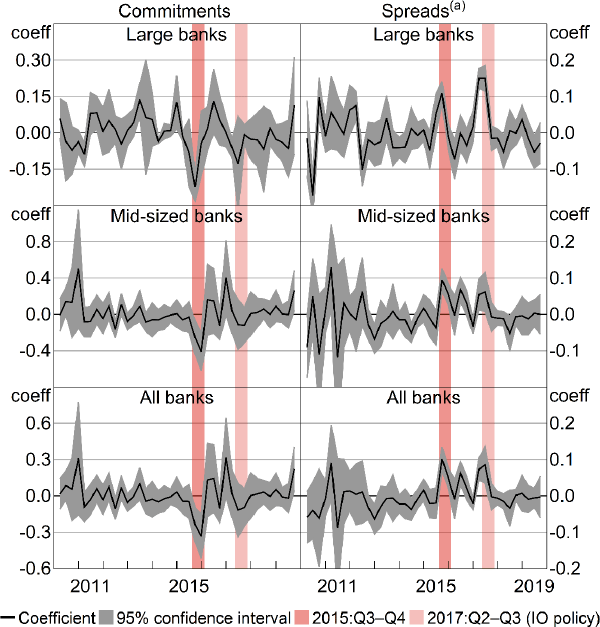
Given that the heterogeneous effect analysis – which applies a more robust identification strategy than the average effect analysis – does not provide causal evidence of a policy effect, this section further explores whether the average policy effect regressions are identifying true policy effects. First, we run the placebo tests described in Section 4.1. Second, we assess potentially confounding trends at the time the policy was implemented. We conclude that the average effect regressions are identifying a true policy effect.
5.4.1 Placebo regressions
The placebo regressions (described in Section 4.1) assess whether the estimated average policy effects could be driven by credit trends that coincide with the policy, but are not caused by the policy. A general interpretation of the results in Sections 5.1 and 5.2 is that, in 2015:Q3 and Q4, mortgage commitments and rates deviate from their typical patterns – as predicted by the regression controls – by a statistically significant degree. The placebo regressions apply the logic that, if these deviations are not caused by the policy, there is a high probability that similar deviations would occur in other periods.
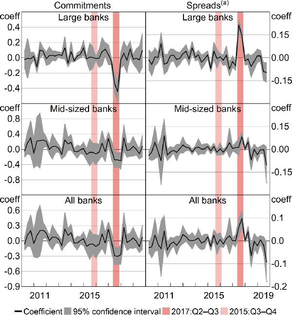
Deviations comparable to the estimated policy effects are absent from other periods. In Figure 6, a deviation is statistically significant at 95 per cent if its grey confidence interval shading does not overlap with the horizontal zero line. There are some statistically significant deviations outside the policy periods, but, excluding those that align with the IO policy (shown in lightest shading), none are the size and statistical significance of the effects during the policy periods. For mid-sized banks, spreads significantly rise between the 2 polices. This is likely a further investor policy reaction, to quell the 2016 pick-up in investor commitments visible in the left panels. The smaller significant deviations in other periods justify caution in relying precisely on the specific coefficient values in Sections 5.1 and 5.2. Overall, however, the placebo results provide confidence that the regressions in Sections 5.1 and 5.2 identify policy effects.
Note: (a) Spreads are between investor rates and occupier rates for P&I mortgages
5.4.2 The potential for coincidental credit trends
Confounding trends could still be driving the estimated average policy effects, if the placebo results are simply a strong coincidence. Any such confounding trends must affect housing investors and housing occupiers differently, because the estimated policy effects show a divergence between investor and occupier mortgages in commitments and spreads. The most plausible driver is therefore housing market conditions. Most other drivers of credit trend deviations, such as factors related to household income, should affect both types of mortgages. This is indeed the identification benefit from using non-treated loan types as a quasi control group.
Housing price growth does decline from mid 2015 for around 6 months (e.g. see Figure 1), but the evidence suggests that, rather than being fully exogenous, this is at least partly caused by banks' policy reactions. Internal RBA work, summarised in RBA (2018), compares regions' housing price behaviour with their proportion of investor ownership.[17] Up to mid 2015, housing price growth is similar in regions with high and low investor ownership. However, from 2015:Q3, once banks begin tightening investor credit, regions with higher proportions of investors experience significantly lower housing price growth than regions with fewer investors.[18] Furthermore, if reverse causality was confounding our analysis – that is, if the housing price growth declines caused a decline in investor demand – then investor rates should experience downward pressure with the downward shift in demand. The fact that investor rates rise is further evidence supporting our identification.
6. Policy Effects of the Interest-only Limit
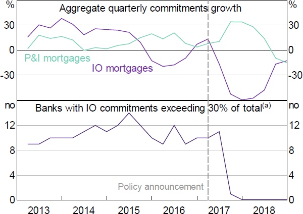
The interest-only mortgage limit, announced at end March 2017, required banks to limit their new IO lending to no more than 30 per cent of total new housing lending. Data are not available for new lending (i.e. mortgage originations), and so we proxy with mortgage commitments. In the aggregate commitments data, the policy effect appears immediate (Figure 7). IO commitments growth falls sharply in 2017:Q2, and in 2017:Q3 and Q4, the number of banks exceeding our proxy of the limit falls to one then zero. This immediate reaction contrasts with the 2-quarter delay in the reaction to the investor policy. Contacts tell us that banks had, by then, developed more capability to control credit growth in targeted products. APRA also provided clearer policy wording. APRA (2019b) writes about the IO policy ‘the experience with the benchmark on lending to investors indicated that the industry would respond most quickly and decisively to a tactical industry-wide regulatory expectation’.
Notes:
The number of banks in the sample varies slightly across periods but is constant from 2016:Q3 to 2018:Q2
(a) May not perfectly align with APRA's assessment of banks meeting the limit
Sources: APRA; Authors' calculations
The results in Sections 6.1 to 6.4 indeed show a faster and neater IO policy reaction than the investor policy reaction. Bank-level growth in IO commitments, and changes in advertised IO rates, react immediately, in 2017:Q2, and large banks substitute into P&I credit one quarter later. Large banks raise advertised IO rates by more than mid-sized banks, and also experience a larger decline in IO commitments growth. Moreover, banks that exceed the IO limit prior to the policy announcement lower their IO commitments growth by significantly more than banks not exceeding the limit. These results are consistent with reports that both banks and APRA benefited from experience with the investor policy while implementing the IO policy.
6.1 Average effects on mortgage commitments
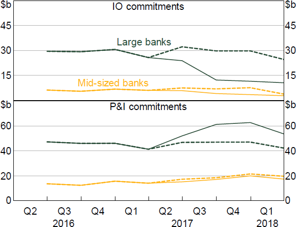
For each sample of banks, the policy significantly reduces targeted credit in the first 3 quarters following the announcement (Table 5). In the full sample, the average bank's IO commitments growth declines 65 percentage points in these 3 quarters (column (a)).[19] Large and mid-sized banks reduce IO commitments growth by around the same overall (columns (d) and (g)), the large banks by a little more. In our commitments proxy, large banks' IO shares tend to exceed the limit by more than mid-sized banks prior to the policy, which explains the larger estimated policy effect for large banks. That is, in the year to 2017:Q1, the average IO share of commitments across large banks lifted from 38 to 41 per cent, while mid-sized banks' same average share lifted from 22 to 24 per cent.
| Sample banks: |
(a) | (b) | (c) | (d) | (e) | (f) | (g) | (h) | (i) | ||
|---|---|---|---|---|---|---|---|---|---|---|---|
| All | Large | Mid-sized | |||||||||
| Mortgage type: | IO | P&I | Total | IO | P&I | Total | IO | P&I | Total | ||
| Policy effects | |||||||||||
| 𝕀(Q2–17) | −0.292*** (0.092) |
−0.099* (0.053) |
−0.166*** (0.042) |
−0.324*** (0.074) |
0.126 (0.099) |
−0.042 (0.052) |
−0.270** (0.110) |
−0.149*** (0.055) |
−0.188*** (0.047) |
||
| 𝕀(Q3–17) | −0.311*** (0.083) |
0.057 (0.041) |
−0.065** (0.025) |
−0.476*** (0.087) |
0.172*** (0.053) |
−0.009 (0.037) |
−0.277*** (0.094) |
0.027 (0.046) |
−0.074*** (0.028) |
||
| 𝕀(Q4–17) | −0.291*** (0.096) |
0.018 (0.053) |
−0.039 (0.051) |
−0.177*** (0.028) |
0.028 (0.036) |
−0.022 (0.023) |
−0.314*** (0.110) |
0.008 (0.062) |
−0.046 (0.061) |
||
| 𝕀(Q1–18) | 0.232 (0.148) |
−0.033 (0.042) |
−0.003 (0.037) |
−0.011 (0.085) |
−0.004 (0.059) |
−0.019 (0.060) |
0.273 (0.171) |
−0.043 (0.050) |
−0.005 (0.043) |
||
| Lagged DVs | 2 | 2 | 2 | 2 | 2 | 2 | 2 | 2 | 2 | ||
| Controls | yes | yes | yes | yes | yes | yes | yes | yes | Yes | ||
| Sample | 788 | 792 | 792 | 168 | 168 | 168 | 620 | 624 | 624 | ||
| Notes: Coefficients from panel regressions, across banks and quarters, of commitments growth on 4 lags of the bank-invariant policy indicator variable. The full equation is in first differences, using Arellano–Bond, with 2 lagged dependent variables to eliminate second order autocorrelation. The control variables are GDP growth, housing price growth, lagged tier 1 capital ratios, lagged deposit funding ratios and a set of seasonal dummy variables. ***, ** and * denote statistical significance at the 1, 5 and 10 per cent levels, respectively. | |||||||||||
In non-targeted credit, large and mid-sized banks' reactions differ, in similar ways to the investor policy reactions. Both curb growth in IO commitments, but only large banks substitute into P&I commitments, so only mid-sized banks reduce total commitments growth. In 2017:Q2 and Q3, large banks experience pick-ups in P&I commitments growth of 13 and 17 basis points, the latter significant, while mid-sized banks experience a significant 15 percentage point decline. The combined effect is that large banks experience no significant change in total commitments growth, while mid-sized banks' total growth declines significantly by around 25 percentage points.
Figure 8 repeats the counterfactuals exercise in Section 5.1 for the IO policy. Large banks' pick-up in commitments for non-targeted (P&I) mortgages is, again, a similar value to their decline in commitments for targeted (IO) mortgages (a bit under $15 billion). Mid-sized banks' non-targeted commitments rise gradually in 2017, but move close to what the estimates suggest would have occurred without the policy.
Sources: APRA; Authors' calculations
6.2 Average effects on advertised interest rates
Large and mid-sized banks both lift IO rates in the first quarter after the policy announcement (Table 6), alongside the declines in IO commitments growth (Section 6.1). Large banks' IO rate rises are larger, in line with their higher IO lending shares prior to the policy (discussed above). At the time, each of the large banks publicly attributed these IO rate rises to the policy (ACCC 2018a). Large and mid-sized banks both reduce IO rates 2 quarters later, when all banks are within our proxy of the limit (Figure 7). The final cumulative effect is still a sizeable IO rate increase – by 34 basis points for the large banks and 16 basis points for the mid-sized banks – which may in part reflect a policy-induced reassessment by banks of the risks of these loans.
The relationships between advertised rate changes and commitments growth, when comparing large and mid-sized banks' reactions, are more intuitive for the IO policy than for the investor policy. Compared to mid-sized banks, large banks initially lift rates by more (in 2017:Q2 and Q3), then lower them by more (in 2017:Q4), and IO commitments growth rates move in the inverse (Table 6, columns (a) and (d); Table 5, columns (d) and (g)). Large banks' non-targeted mortgage commitments, however, appear less sensitive to rates than those of mid-sized banks. In 2017:Q2, both types of banks raise P&I rates, but only mid-sized banks' P&I commitments growth falls.[20] However, this could potentially be explained by large banks' heavier use of rate discounting, which would cause overstated estimates of the true changes in mortgage rates.
| Sample banks: |
(a) | (b) | (c) | (d) | (e) | (f) | |
|---|---|---|---|---|---|---|---|
| Large | Mid-sized | ||||||
| Dependent variable: | IO | P&I | Difference | IO | P&I | Difference | |
| 𝕀(Q2–17) | 0.325*** (0.028) |
0.103*** (0.020) |
0.222*** (0.016) |
0.115*** (0.036) |
0.095*** (0.020) |
0.020 (0.028) |
|
| 𝕀(Q3–17) | 0.106*** (0.031) |
−0.048** (0.022) |
0.154*** (0.015) |
0.097** (0.044) |
0.010 (0.043) |
0.087*** (0.017) |
|
| 𝕀(Q4–17) | −0.090*** (0.029) |
−0.084*** (0.026) |
−0.006 (0.011) |
−0.044** (0.018) |
−0.050** (0.018) |
0.007* (0.004) |
|
| 𝕀(Q1–18) | −0.019 (0.028) |
−0.027 (0.024) |
0.008 (0.014) |
0.043 (0.031) |
−0.010 (0.021) |
0.054*** (0.017) |
|
| Fixed effects | Bank | Bank | Bank | Bank | Bank | Bank | |
| Other controls | yes | yes | yes | yes | yes | yes | |
| R squared | 0.327 | 0.212 | 0.277 | 0.087 | 0.111 | 0.052 | |
| Sample | 164 | 164 | 164 | 501 | 500 | 496 | |
| Notes: Coefficients from panel regressions, across banks and quarters, of change in advertised mortgage rates on 4 lags of the bank-invariant policy indicator variable. All mortgage rates are on investor mortgages. The control variables are GDP growth, housing price growth, lagged tier 1 capital ratios, lagged deposit funding ratios and a set of seasonal dummy variables. Bank fixed effects are included. Standard errors are clustered at the quarter level for the large bank regressions, and at the bank and quarter levels for the mid-sized bank regressions. ***, ** and * denote statistical significance at the 1, 5 and 10 per cent levels, respectively. | |||||||
6.3 Heterogeneous IO-policy effects
In contrast to the investor policy, banks' reactions to the IO policy are clearly related to whether they exceed the limit. In 2017:Q3, banks above the limit reduce IO commitments growth by 27 percentage points more than banks below the limit (Table 7, column (b)).[21] In the same quarter, the linear treatment measure shows that, for every 10 percentage points further above the limit, a bank reduces its IO commitments growth by 14 percentage points more (column (a)).[22] As opposed to the lack of differentiation between banks below and above the threshold seen in Section 6.1, for the IO benchmark banks above react differently to banks below. In addition, banks above the limit have a significantly larger pickup in P&I commitments growth than banks below (columns (c) and (d)). The strong substitution effect for banks above the limit is not surprising, because raising P&I lending is also a way to meet the proportion-based limit on IO lending.
| Dependent variable: |
(a) | (b) | (c) | (d) | (e) | (f) | (g) | (h) | ||||
|---|---|---|---|---|---|---|---|---|---|---|---|---|
| Commitments growth | Rate changes | |||||||||||
| Mortgage type: | IO | P&I | IO | P&I | ||||||||
| Treatment function: | Linear | Binary | Linear | Binary | Linear | Binary | Linear | Binary | ||||
| 𝕀(Q2–17) ×Treatment |
−0.549 (0.496) | −0.095 (0.073) | 1.008*** (0.120) | 0.237*** (0.045) | 0.460*** (0.142) | 0.166*** (0.036) | −0.023 (0.097) | −0.051* (0.026) | ||||
| 𝕀(Q3–17) ×Treatment |
−1.440*** (0.444) | −0.272*** (0.075) | 0.564*** (0.098) | 0.216*** (0.033) | −0.182 (0.269) | −0.055 (0.058) | −0.027 (0.098) | 0.017 (0.019) | ||||
| 𝕀(Q4–17) ×Treatment |
−0.738 (0.761) | 0.029 (0.086) | 0.355 (0.237) | 0.084 (0.056) | −0.170 (0.155) | −0.001 (0.032) | −0.024 (0.065) | 0.006 (0.010) | ||||
| 𝕀(Q1–18) ×Treatment |
−3.079*** (0.803) | 0.012 (0.099) | 0.168 (0.198) | 0.318*** (0.029) | −0.162 (0.143) | 0.000 (0.000) | −0.023 (0.039) | −0.002 (0.004) | ||||
| Fixed effects | Bank & quarter | Bank & quarter | Bank & quarter | Bank & quarter | Bank & quarter | Bank & quarter | Bank & quarter | Bank & quarter | ||||
| Bank controls | yes | yes | yes | yes | yes | yes | yes | yes | ||||
| R squared | 0.368 | 0.359 | 0.346 | 0.346 | 0.210 | 0.211 | 0.727 | 0.728 | ||||
| Sample | 871 | 871 | 874 | 874 | 214 | 214 | 654 | 654 | ||||
| Notes: Coefficients from regressing commitments growth, or change in advertised rates, on 4 lags of the bank-invariant policy indicator variable, each interacted with a ‘treatment’ measure of the bank's distance from the policy limit 2 quarters earlier. The 2 alternative treatment measures are ‘Linear’, equal to the bank's year-ended investor mortgage growth rate (as a decimal) minus 0.1, and ‘Binary’, an indicator for if the bank was exceeding the limit. The regressions include bank and quarter fixed effects. Bank-level controls (capital and deposits) are also included. Standard errors are clustered at the bank and quarter levels. ***, ** and * denote statistical significance at the 1, 5 and 10 per cent levels, respectively. | ||||||||||||
The heterogeneous effect on rates is also clear. In 2017:Q2, every 10 percentage points above the limit translates to a 5 basis point larger IO rate increase (Table 7, column (e)). On average, banks above the limit raise IO rates by 17 basis points more than banks below (column (f)). Also in 2017:Q2, banks above the limit raise P&I rates by 5 basis points less than banks below (column (h)), but there is no significant effect when measuring distance from the limit as a linear rather than binary variable. IO rate effects in subsequent quarters tend to backtrack, but the changes are smaller than the initial policy effects and the coefficients are not significant.
6.4 Placebo regressions
The placebo regression results provide further evidence, in addition to the heterogeneous effect regressions, that the estimated policy effects in Sections 6.1 and 6.2 are true policy effects. In all of the placebo regressions, there are no deviations outside the policy periods that have the size and statistical significance of the estimated policy effects (Figure 9).
Note: (a) Spreads are between IO rates and P&I rates for investor mortgages
7. Other Mortgage Market Outcomes
This section analyses policy effects on other outcomes of interest, and the cyclicality of mortgage commitments throughout the sample. The first part shows how APRA's soft guidance on LVRs interacted with the mortgage growth limits. The second part looks at how the policies affected aggregate variables related to total credit growth, banking market share and banks' mortgage interest income. The third part discusses an unintended side effect of the investor policy – customers switching the classification of their loan from investor to occupier. The fourth part discusses some results for mortgage commitments behaviour throughout the sample.
7.1 Policy effects by loan-to-valuation ratio
The two macroprudential limits were accompanied by guidance from APRA that banks should manage their high-LVR lending. When announcing the investor policy, LVRs were only mentioned briefly. APRA stated that it would generally lift scrutiny over higher risk lending, and gave several examples of higher risk lending that included ‘lending at high loan-to-valuation ratios’ (APRA 2014). When announcing the IO policy, the advice was more explicit. Banks were asked to:
… place strict internal limits on the volume of interest-only lending at loan-to-valuation ratios (LVRs) above 80 per cent; and
… ensure there is strong scrutiny and justification of any instances of interest-only lending at an LVR above 90 per cent … (APRA 2017).
This subsection separates mortgage commitments into 3 LVR buckets and analyses the policy effects separately for each. This serves 2 purposes. First, it tests whether the results in Sections 5 and 6 could simply be picking up APRA's guidance on LVRs, given that targeted loan types can have higher LVRs. If this was the case, then regressions that hold LVRs constant would show the same policy effects in targeted and non-targeted loan types. Second, it provides additional understanding of how the overall policy packages affected mortgages of different LVRs.
The analysis is approached with some modifications to the commitments growth regressions in Sections 5 and 6. To distinguish commitments by LVR, we add an LVR dimension ( l ) to the dataset. This basically means creating 3 datasets for different LVR buckets – LVR ≤ 80%; 80% < LVR ≤ 90%; and LVR > 90% – and stacking them together to form a bank-quarter-LVR-level dataset. The policy effects are then estimated separately for each LVR bucket, by interacting the policy indicator variable with an indicator variable for the LVR level. To capture the results in a concise set of coefficients, the 4 policy indicator lags used in the previous regressions are replaced with a single policy indicator that equals one in both of the 2 quarters in which the policies had most effect, as informed by the previous results (i.e. for the investor policy, 2015:Q3 and Q4, and for the IO policy, 2017:Q2 and Q3). Instead of using first differences and the Arrellano-Bond instrumental variables method, the regressions include fixed effects at the bank × LVR bucket level. Data are not available for IO commitments, so for both policies, we compare investor and occupier commitments, which means the results for IO policy effects are less reliable.
Specifically, the regression equations are
The results show that the policy effects found in Sections 5 and 6 are not simply capturing LVR effects (Table 8). Within each LVR bucket, the policy effect coefficients are consistently more negative for investor commitments than for occupier commitments. In particular, the effect of investor limit on investor commitments is strongest in the highest LVR bucket, while in that bucket there is virtually no policy effect on occupier commitments.
| Sample banks: |
(a) | (b) | (c) | (d) | |
|---|---|---|---|---|---|
| Large | Mid-sized | ||||
| Commitments type: | Investor | Occupier | Investor | Occupier | |
| Investor policy regressions | |||||
| 𝕀(LVR ≤ 80)×𝕀(Invpolicy) | −0.189 (0.122) |
0.154* (0.091) |
−0.263** (0.116) |
0.016 (0.081) |
|
| 𝕀(80 < LVR ≤ 90)×𝕀(Invpolicy) | −0.095 (0.122) |
0.199** (0.091) |
−0.298** (0.120) |
−0.067 (0.082) |
|
| 𝕀(LVR > 90)×𝕀(Invpolicy) | −0.511*** (0.123) |
0.004 (0.091) |
−0.405*** (0.128) |
−0.019 (0.081) |
|
| R squared | 0.116 | 0.084 | 0.094 | 0.066 | |
| Sample | 528 | 528 | 1,811 | 1,996 | |
| IO policy regressions | |||||
| 𝕀(LVR ≤ 80)×𝕀(IOpolicy) | −0.033 (0.124) |
0.032 (0.091) |
−0.094 (0.103) |
−0.016 (0.071) |
|
| 𝕀(80 < LVR ≤ 90) × 𝕀(IO policy) | −0.107 (0.124) |
0.044 (0.091) |
−0.198* (0.107) |
−0.067 (0.071) |
|
| 𝕀(LVR > 90)×𝕀(IOpolicy) | −0.192 (0.124) |
−0.022 (0.091) |
−0.300** (0.123) |
−0.193*** (0.072) |
|
| R squared | 0.087 | 0.072 | 0.088 | 0.069 | |
| Sample | 528 | 528 | 1,811 | 1,996 | |
| Fixed effects | Bank × LVR | Bank × LVR | Bank × LVR | Bank × LVR | |
| Other controls | yes | yes | yes | yes | |
| Notes: Coefficients from regressions at the bank–quarter–LVR bucket level, as specified in Equation (4). The controls include 2 lagged dependent variables, to be consistent with the regressions in Sections 5 and 6. The lagged dependent variables deal with any autocorrelation, in the same manner as in the Section 5 and 6 regressions, so the standard errors are not additionally clustered. ***, ** and * denote statistical significance at the 1, 5 and 10 per cent levels, respectively. | |||||
Notwithstanding this, the policies do have a significant effect on the LVR distribution, in line with APRA's guidance. Declines in targeted mortgages are concentrated in the highest LVR bucket, and rises in non-targeted mortgages are concentrated in lower LVR buckets. Mid-sized banks reduce low-LVR credit in targeted mortgages more so than large banks, but the strongest effect for mid-sized banks is still clearly in the highest LVR loans. APRA's guidance on LVRs appears to have interacted with the mortgage limits by determining, within each type of mortgage, at what LVRs the reactions occur.
7.2 Policy effects on aggregate variables
This section analyses policy effects on aggregate variables of interest. The analysis uses time series regressions that regress the outcome variable on various controls, including lagged dependent variables. The exact specifications are discussed in each subsection, and resemble Equations (1) and (2) with the cross-section collapsed into a single series. The time series samples are small, so we report these results in placebo regression figures as in Sections 5.4.1 and 6.4. These sets of estimates nest the estimated policy effects, which are the ‘placebo’ coefficients for the quarters when the policies were actually implemented. Comparing the full set of ‘trend deviation’ coefficients also indicates the reliability of the estimated policy effects, in the same manner as the placebo regressions presented earlier. To reiterate, the results show a statistically significant policy effect if, during the policy quarters, the coefficient's 95 per cent confidence interval is fully above or below zero. The fewer significant effects outside the policy period, the more robust any estimated policy effects are.
7.2.1 Effects on aggregate housing and business credit growth
The results in Sections 5 and 6 analyse bank-level credit reactions, but do not measure the policy effect on total housing credit, because those regressions weight each of the sample banks equally. To formally test for effects on credit aggregates we estimate
The dependent variable CreditGrth takes on 4 definitions: total investor housing credit, total occupier housing credit, total (domestic) housing credit and total (domestic) business credit.[23] (Reliable aggregates for IO and P&I housing credit are not available.) As discussed above, this regression is repeated multiple times while rolling the quarter in 𝕀(quarter)t across all quarters from 2010 to 2019. The vector Controlst includes GDP growth, housing price growth, the first difference of the cash rate and its first lag, the average capital ratio across sample banks, the average deposit ratio across sample banks, and a set of seasonal indicators. These variables are defined as in Section 3.2.
The raw data and the regression results both suggest that the policies had little effect on banks' total housing credit (Figure 10, left panels). While each policy coincided with a decline in investor credit growth and a pick-up in occupier credit growth, total housing credit growth remained relatively flat. (Aggregate credit growth data are not available for IO mortgages, but, as evident in Figure 1, the IO share of investor loans is higher than that of occupier loans.) Credit growth dropped just after the investor policy period, but this was driven by a decline in occupier growth. APRA (2019b) also concludes that, for the investor policy, the aggregate trend in housing credit growth remained broadly unchanged.
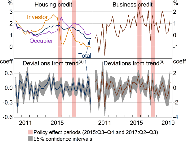
Note: (a) Coefficient estimates from rolling ‘placebo’ regressions, described in text
Sources: Authors' calculations; RBA Statistical table D1 Growth in Selected Financial Aggregates
Next, CreditGrtht is defined as banks' total domestic business credit growth. The policies could feasibly affect business credit for at least 2 reasons. Banks might substitute away from the targeted mortgage type and into business credit, similar to the effect for large banks in occupier credit during the first policy. This would cause a pick-up in business credit. Alternatively, business credit could be neglected as banks concentrate more resources on controlling their mortgage portfolio. This would cause a decline in business credit.
There is evidence for a pick-up in business credit growth during the investor policy (Figure 10, bottom right panel). The trend deviation is larger and has a higher significance level than any trend deviation coefficients since 2011. This result is consistent with a substitution into business credit by banks compensating for less investor mortgage origination. There is no significant effect for the IO policy.
7.2.2 Effects on market concentration
Sections 5 and 6 show that large banks substitute into non-targeted mortgage types while mid-sized banks do not. This section tests whether the different responses resulted in the large banks increasing their mortgage market share relative to the mid-sized banks. We conclude that large banks' IO policy-induced substitution into P&I loans likely had a positive single-quarter effect on their mortgage market share relative to the 20 or so mid-sized banks in our sample, and this was at the expense of large banks' mortgage interest income.
The analysis re-estimates Equation (5), but replaces CreditGrtht with 1 of 2 measures of large banks' market share: their mortgage interest income (MII) as a proportion of the total across sample banks; and their quarterly dollar change in mortgage credit outstanding as a proportion of the total across sample banks.[24] For the MII regressions, the cash rate control variables are included as levels rather than first differences, because mortgage interest rates are closely related to the cash rate level. Both dependent variables are sourced from the APRA dataset noted in Section 3.1.
Large banks' MII share significantly drops during the IO policy period, in 2017:Q2 Figure 11, bottom left panel). This is likely driven by their bigger decline in IO commitments growth relative to midsized banks (Section 6.1), which reflects their higher share of IO commitments prior to the policy. The effect appears temporary: large banks' MII share is above trend in 2017:Q3, but not significantly (bottom left panel), and the rebound is visible in the raw data (top left panel).
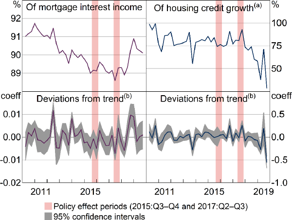
Notes:
(a) Large banks' quarterly change in credit (in $) divided by all banks' quarterly change in credit
(b) Coefficient estimates from rolling ‘placebo’ regressions, described in text
Sources: APRA; Authors' calculations; RBA
Large banks' share of credit growth across sample banks significantly rises in 2017:Q3 before dropping again (Figure 11, bottom right panel). The timing matches their substitution into P&I commitments growth (Table 5), and may be the driver of their rebound in MII share. The effect again appears temporary: their share of credit growth drops and is below trend in all of the following few quarters (right panels).
The investor policy has no statistically significant effect on large banks' share of MII or of mortgage credit growth (Figure 11, bottom panels). The raw data show that large banks' share of MII picks up after the investor policy (top left panel), but the regression results show that it is not a statistically significant deviation from trend (bottom left panel), and therefore likely unrelated to the policy.
7.2.3 Effects on banks' pricing power
The Australian Government Productivity Commission (PC) has criticised the policies for their competition implications. PC (2018, p 180) writes:
Under the benchmark interventions, any ADI charging a materially lower interest rate than its competitors would receive an outsized number of loan applications that, if approved, could result in it breaching APRA's growth limit for the investor segment. As a result, ADIs increased their pricing for investor and interest-only lending — including both new and existing loans — or temporarily discontinued cheaper products …
Notwithstanding this, PC (2018) also concludes that swift action by APRA was appropriate and that APRA's proposed risk weight changes are an appropriate tool going forward. The ACCC has reached similar conclusions to the PC. ACCC (2018a, p 42) writes:
While APRA's interest-only benchmark had the objective of contributing to financial system stability, we find it lessened price competition for interest-only lending. We consider that the benchmark provided the opportunity for the banks to synchronise their significant increases to interest-only rates during the price monitoring period, at a significant cost to those borrowers.
Ultimately, the PC and ACCC concerns are that the policies lifted banks' ability to extract surplus value from customers (in a microeconomic sense), by inducing a softening of pricing competition between banks. To analyse this, we look at reactions in banks' total MII. A change in prices alone does not reveal competition effects, because the price change could be exogenously driven – for example, by new information about loan riskiness or potential future funding costs – and customers' demand reductions could still be consistent with a competitive market, with substitution into competing products. The main difference between a competitive and a monopolistic market is in the price elasticity of demand (e.g. Dixit and Stiglitz 1977). The implication is that, if a price rise is driven by a lift in monopolistic power, income should also pick up, with the monopolist benefiting from the combination of the price rise and customers' demand insensitivity.
To test whether the policies caused a pick-up in MII, we re-estimate Equation (5) but replace CreditGrtht with the cross-sectional sum of sample banks' housing interest income (from the same APRA dataset). As in the MII analysis in Section 7.2.2, the cash rate control variables are included as levels rather than first differences.[25]
MII is significantly above trend in both of the IO policy quarters (Figure 12, bottom panel). There is also a positive significant trend deviation in 2016:Q4, which could have been a delayed reaction to the investor policy, but this is less conclusive and is not apparent in the raw data (top panel). Either way, the significant deviations in the IO policy period are consistent with the hypothesis that the IO policy temporarily lifted banks' monopolistic pricing power. Combining this result with the results in Section 7.2.2 suggests that the monopolistic benefit went to mid-sized banks initially (in 2017:Q1), before spreading across all banks (in 2017:Q2). It is worth noting, however, that competition and financial stability can conflict with each other. For example, APRA's letter to ADIs about the investor policy notes that strong competition in the housing market was pushing lending standards down (APRA 2014). The potential conflict is also well established in the empirical and theoretical banking literature (e.g. Freixas and Rochet 2008; Berger, Klapper and Turk-Ariss 2017).
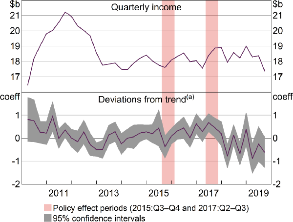
Note: (a) Coefficient estimates from rolling ‘placebo’ regressions, described in text
Sources: APRA; Authors' calculations
7.3 Loan-type switching
When the investor policy was implemented, regulators observed that many existing borrowers were reclassifying themselves from investor to occupier. That is, borrowers who were investors at origination were notifying their bank that they were now occupiers. The policy caused incentives for borrowers to do this, to receive a lower interest rate (Section 5.2). Banks may have also initially thought that this loan-type switching would help them to meet the investor credit growth limit, although APRA has noted that it measured credit growth by looking through loan-type switching (APRA 2019b). APRA began asking banks for monthly data on loan-type switching in July 2015 (Figure 13). From July to October 2015, credit growth from loan-type switching dominated standard credit growth.
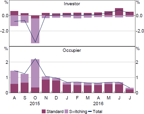
Source: RBA
This policy-induced loan-type switching is one of the reasons we use mortgage commitments as the dependent variable for our credit quantity regressions. Commitments should be less affected than credit growth by loan-type switching, because customers typically do not have to make a new loan application to switch their loan type within the same bank. However, commitments may not completely remove loan-type switching effects, because some customers could go to the extra effort of switching by applying for refinancing at a new bank, potentially to take advantage of lower rates at that bank. To the extent that this occurred, our investor policy effects may be overestimated.
7.4 The cyclicality of mortgage products
The commitments regressions in Sections 5.1 and 6.1 include macroeconomic control variables whose coefficients are informative about the general behaviour of commitments growth. However, those regressions group mortgage types together within the targeted and non-targeted categories, which is appropriate for analysing policy effects, but less so for analysing general mortgage behaviour. Here we report control coefficient estimates that are more definitive by running separate regressions on the 4 mortgage subtypes: occupier P&I, occupier IO, investor P&I and investor IO. These regressions re-estimate Equation (1) (with different definitions of m ), but include all 8 policy indicators in each regression (4 each for the investor and IO policies).
Housing prices correlate with investor commitments and IO commitments, but not with occupier P&I commitments (Table 9). This may suggest that speculative demand for housing is in part driven by extrapolation of recently observed house prices (e.g. extrapolative expectations are discussed in Armona, Fuster and Zafar (2019)), in line with prevailing views on the Australian housing market (e.g. APRA 2019b). This effect is stronger for large banks than for mid-sized banks; we do not speculate on why. Basten and Koch (2015) find a positive causal relationship of housing prices on mortgage demand. Our findings build on their results by showing that this holds true only for housing investors, at least in Australia. The lack of relationship with occupier P&I credit, which in Australia is the largest housing credit category (Figure 1), is consistent with the cross-country panel findings in Kearns, Major and Norman (2020) that, in aggregate, housing prices do not have a positive effect on household debt.
| Dependent variable: |
(a) | (b) | (c) | (d) | (e) | (f) | (g) | (h) | |||
|---|---|---|---|---|---|---|---|---|---|---|---|
| Occupier P&I | Investor P&I | Occupier IO | Investor IO | ||||||||
| Sample banks: | Large | Mid-sized | Large | Mid-sized | Large | Mid-sized | Large | Mid-sized | |||
| GDP | 0.055 (0.043) |
0.101*** (0.034) |
0.042* (0.025) |
0.111* (0.064) |
−0.005 (0.051) |
0.004 (0.070) |
−0.028 (0.039) |
0.055 (0.043) |
|||
| Housing prices | 0.003 (0.007) |
−0.001 (0.008) |
0.036*** (0.009) |
0.003 (0.011) |
0.015*** (0.004) |
0.017* (0.010) |
0.018* (0.011) |
0.003 (0.007) |
|||
| Lagged DVs | 2 | 2 | 2 | 2 | 2 | 2 | 2 | 2 | |||
| Policy indicators | 8 | 8 | 8 | 8 | 8 | 8 | 8 | 8 | |||
| Other controls | yes | yes | yes | yes | yes | yes | yes | Yes | |||
| Sample | 168 | 624 | 168 | 621 | 168 | 620 | 168 | 168 | |||
| Notes: Coefficients from panel regressions, across banks and quarters, of granular categories of commitments growth on quarterly GDP growth and quarterly housing price growth. The full equation is in first differences, using Arellano–Bond, with 2 lagged dependent variables (to eliminate second order autocorrelation). Other controls include all 8 policy indicator variables, seasonal indicators and the bank-level control variables (capital and deposits). For the mid-sized banks' regression of occupier IO commitments, only 2 seasonal indicators are used, to avoid multicollinearity with instruments. ***, ** and * denote statistical significance at the 1, 5 and 10 per cent levels, respectively. | |||||||||||
GDP correlates with P&I commitments but not IO commitments (Table 9), and the effect is stronger for mid-sized banks than for large banks. Income is an intuitive driver of general mortgage commitments through its link with borrowing capacity. A plausible explanation for its lack of relationship with IO commitments is that IO commitments have their own structural drivers. For example, between 2011 and 2014, when aggregate IO lending was growing strongly and housing price growth was picking up, GDP growth was trending downwards (Figure 1). This structural shift in IO lending is also noted in ASIC (2015).
8. Conclusions
This paper shows that APRA's 2014 and 2017 macroprudential credit limits quickly reduced housing credit growth in the targeted mortgage products. To conclude, we reiterate how the paper's empirical findings align with the 3 key results outlined in the Introduction.
1. Banks met the credit growth limits by raising interest rates, enabled by the policies. The policies caused banks to raise rates on targeted mortgage types (Sections 5 and 6). This was to some degree intended, because banks were viewed as underpricing the risk inherent in those loans (RBA 2018). The rise in mortgage rates has already been shown: the ACCC and PC examine this in their analysis of competition in the Australian mortgage market (ACCC 2018a, 2018b; PC 2018). Our results add statistical evidence of a policy effect to their conclusions, quantify the rate reactions for different banks, and show that, for the investor policy, banks' credit quantity reactions were also driven by factors other than interest rate changes (Section 5.2).
ACCC (2018a, 2018b) conclude that some of the rate rises reflected a policy-induced softening of price competition. Our results indicate that this was in part true for the IO policy, because banks' mortgage interest income picked up above model-implied values temporarily during this period (Section 7.2.3). There were also rate rises on non-targeted mortgages after the investor policy, but banks indicated these were driven by funding costs (Section 5.2). The temporary softening of pricing competition, while a negative consequence in itself, was possibly a worthwhile cost, given that the policy appears to have achieved its financial stability objectives.
2. Banks' reactions to the limits depended on their size. Large banks substituted into non-targeted mortgage types by, at least in part, reducing rates on those mortgages (Sections 5.2 and 6.2), while mid-sized banks lowered rates on non-targeted mortgages but experienced no substitution. In turn, large banks' average mortgage growth did not significantly change, while midsized banks' average mortgage growth significantly declined (Sections 5.1 and 6.1). However, the positive effect on large banks' share, among the sample banks, was only small and short-lived, seemingly at the expense of their interest income (Section 7.2.2). It is not entirely clear why large banks substituted and mid-sized banks did not, but it is plausible that large banks' operational systems were more flexible. Future work could explore this.
3. Practical implementation difficulties complicated the policy effects. The reactions to the investor policy do not neatly align with a theoretical representation of banks choosing new credit growth targets and shifting to them. Practical difficulties complicated the outcomes. The reaction to the investor policy had a 2-quarter delay (Section 5.1), some mid-sized banks had difficulty controlling their investor credit flows (Section 5.2) and several banks that were not exceeding the investor limit contracted lending seemingly unnecessarily (Section 5.3). The delay was partly caused by these control difficulties, but, as contacts tell us, partly also due to uncertainty about how strictly and quickly the limit would be applied, and around how the limit was defined (Section 5). For example, many investor mortgagees reacted to the rate rises by telling their bank they were actually occupiers (Section 7.3), which complicated credit growth calculations.
In contrast, banks' reactions to the IO policy were immediate and more closely related to whether they exceeded the limit (Section 6). It appears that banks improved their systems while reacting to the investor policy, including by developing price differentiation capabilities. APRA was also intentionally more explicit in its expectations for the IO policy.
Final comments. The overarching objective of the policies was to strengthen financial stability given the pre-existing economic environment. The goal of this paper is to examine banks' reactions, rather than to explicitly gauge the policy success, but our results are consistent with the objective being achieved. Commitments growth in the targeted mortgage products – products that were judged to be contributing to systemic risk at the time – dropped markedly, after growing strongly prior to the policies. Banks now charge higher spreads on the mortgage products that were targeted, and APRA will soon reform capital risk weightings to account for the differential in systemic risk contributions across mortgage types.
References
Acharya VV, K Bergant, M Crosignani, T Eisert and FJ McCann (2020), ‘The Anatomy of the Transmission of Macroprudential Policies’, NBER Working Paper No 27292.
Adelino M, A Schoar and F Severino (2016), ‘Loan Originations and Defaults in the Mortgage Crisis: The Role of the Middle Class’, The Review of Financial Studies, 29(7), pp 1635–1670.
Aiyar S, CW Calomiris and T Wieladek (2014), ‘Does Macro-Prudential Regulation Leak? Evidence from a UK Policy Experiment’, Journal of Money, Credit and Banking, 46(s1), pp 181–214.
Alam Z, A Alter, J Eiseman, G Gelos, H Kang, M Narita, E Nier and N Wang (2019), ‘Digging Deeper—Evidence on the Effects of Macroprudential Policies from a New Database’, IMF Working Paper No WP/19/66.
Araujo J, M Patnam, A Popescu, F Valencia and W Yao (2020), ‘Effects of Macroprudential Policy: Evidence from over 6,000 Estimates’, IMF Working Paper No WP/20/67.
Armona L, A Fuster and B Zafar (2019), ‘Home Price Expectations and Behaviour: Evidence from a Randomized Information Experiment’, The Review of Economic Studies, 86(4), pp 1371–1410.
Armstrong J, H Skilling and F Yao (2019), ‘Loan-to-Value Ratio Restrictions and House Prices: Micro Evidence from New Zealand’, Journal of Housing Economics, 44, pp 88–98.
ACCC (Australian Competition and Consumer Commission) (2018a), Residential Mortgage Price Inquiry: Final Report, Australian Competition and Consumer Commission, Canberra.
ACCC (2018b), ‘Residential Mortgage Price Inquiry: Interim Report’.
APRA (Australian Prudential Regulation Authority) (2014), ‘Reinforcing Sound Residential Mortgage Lending Practices’, Letter to authorised deposit-taking institutions, 9 December.
APRA (2017), ‘Further Measures to Reinforce Sound Residential Mortgage Lending Practices’, Letter to authorised deposit-taking institutions, 31 March.
APRA (2019a), ‘APG 223 Residential Mortgage Lending’, Prudential Practice Guide, July.
APRA (2019b), ‘Review of APRA's Prudential Measures for Residential Mortgage Lending Risks’, Information Paper, 29 January.
APRA (2020), ‘A More Flexible and Resilient Capital Framework for ADIs’, Discussion Paper, 8 December.
ASIC (Australian Securities and Investments Commission) (2015), ‘Review of Interest-Only Home Loans’, Report 445. Available at <https://asic.gov.au/regulatory-resources/find-a-document/reports/rep-445-review-of-interest-only-home-loans/>.
Basten C (2020), ‘Higher Bank Capital Requirements and Mortgage Pricing: Evidence from the Counter-Cyclical Capital Buffer’, Review of Finance, 24(2), pp 453–495.
Basten C and C Koch (2015), ‘The Causal Effect of House Prices on Mortgage Demand and Mortgage Supply: Evidence from Switzerland’, Journal of Housing Economics, 30, pp 1–22.
Bender R and S Lange (2001), ‘Adjusting for Multiple Testing—When and How?’, Journal of Clinical Epidemiology, 54(4), pp 343–349.
Berger AN, LF Klapper and R Turk-Ariss (2017), ‘Bank Competition and Financial Stability’, in JA Bikker and L Spierdijk (eds), Handbook of Competition in Banking and Finance, Edward Elgar Publishing, Cheltenham, pp 185–204.
Borio C and P Lowe (2002), ‘Asset Prices, Financial and Monetary Stability: Exploring the Nexus’, BIS Working Papers No 114.
Cerutti E, S Claessens and L Laeven (2017), ‘The Use and Effectiveness of Macroprudential Policies: New Evidence’, Journal of Financial Stability, 28, pp 203–224.
Debelle G (2019), ‘Housing and the Economy’, Address given at the CFA Societies Australia Investment Conference ‘Beyond Disruption: The Changing Face of Investment Management’, Sydney, 17 October.
DeFusco AA, S Johnson and J Mondragon (2020), ‘Regulating Household Leverage’, The Review of Economic Studies, 87(2), pp 914–958.
Dell'Ariccia G, D Igan, L Laeven and H Tong with B Bakker and J Vandenbussche (2012), ‘Policies for Macrofinancial Stability: How to Deal with Credit Booms’, IMF Staff Discussion Note SDN/12/06.
Dixit AK and JE Stiglitz (1977), ‘Monopolistic Competition and Optimum Product Diversity’, The American Economic Review, 67(3), pp 297–308.
Dobson C (2020), ‘Assessing the Effects of Housing Policy Measures on New Lending in Australia’, in Measuring the Effectiveness of Macroprudential Policies Using Supervisory Bank-Level Data, BIS Papers No 110, Bank for International Settlements, Basel, pp 17–30.
Ellis L and C Littrell (2017), ‘Financial Stability in a Low Interest Rate Environment: An Australian Case Study’, in J Hambur and J Simon (eds), Monetary Policy and Financial Stability in a World of Low Interest Rates, Proceedings of a Conference, Reserve Bank of Australia, Sydney, pp 135–154.
Foote CL, L Loewenstein and PS Willen (2021), ‘Cross-Sectional Patterns of Mortgage Debt during the Housing Boom: Evidence and Implications’, The Review of Economic Studies, 88(1), pp 229–259.
Freixas X and J-C Rochet (2008), Microeconomics of Banking, 2nd edn, The MIT Press, Cambridge.
Guiso L, A Pozzi, A Tsoy, L Gambacorta and PE Mistrulli (forthcoming), ‘The Cost of Steering in Financial Markets: Evidence from the Mortgage Market, Journal of Financial Economics.
Jiménez G, S Ongena, J-L Peydró and J Saurina (2017), ‘Macroprudential Policy, Countercyclical Bank Capital Buffers, and Credit Supply: Evidence from the Spanish Dynamic Provisioning Experiments, Journal of Political Economy, 125(6), pp 2126–2177.
Kearns J, M Major and D Norman (2020), ‘How Risky is Australian Household Debt?’, RBA Research Discussion Paper No 2020-05.
Kent C (2018), ‘The Limits of Interest-Only Lending’, Address to the Housing Industry Association Breakfast, Sydney, 24 April.
Kuttner KN and I Shim (2016), ‘Can Non-Interest Rate Policies Stabilize Housing Markets? Evidence from a Panel of 57 Economies’, Journal of Financial Stability, 26, pp 31–44.
PC (Productivity Commission) (2018), Competition in the Australian Financial System, Productivity Commission Inquiry Report No 89, Productivity Commission, Canberra.
Peydró J-L, F Rodriguez-Tous, J Tripathy and A Uluc (2020), ‘Macroprudential Policy, Mortgage Cycles and Distributional Effects: Evidence from the UK’, Bank of England Staff Working Paper No 866.
RBA (Reserve Bank of Australia) (2018), ‘Assessing the Effects of Housing Lending Policy Measures’, Financial Stability Review, October, pp 75–88.
Reinhart CM and KS Rogoff (2011), ‘From Financial Crash to Debt Crisis’, The American Economic Review, 101(5), pp 1676–1706.
Richter B, M Schularick and P Wachtel (2021), ‘When to Lean against the Wind’, Journal of Money, Credit and Banking, 53(1), pp 5–39.
Roberts MR and TM Whited (2013), ‘Endogeneity in Empirical Corporate Finance’, in GM Constantinides, M Harris and RM Stulz (eds), Handbook of the Economics of Finance: Volume 2A Corporate Finance, Handbooks in Economics, Elsevier, Amsterdam, pp 493–572.
Schularick M and AM Taylor (2012), ‘Credit Booms Gone Bust: Monetary Policy, Leverage Cycles, and Financial Crises, 1870–2008’, The American Economic Review, 102(2), pp 1029–1061.
Upper C (2017), ‘Macroprudential Frameworks, Implementation and Relationship with Other Policies’, in Macroprudential Frameworks, Implementation and Relationship with Other Policies, BIS Papers No 94, Bank for International Settlements, Basel, pp 1–5.
Copyright and Disclaimer Notice
RP Data Pty Ltd trading as CoreLogic Asia Pacific Disclaimer Notice
The following Disclaimer Notice applies to content that uses data from CoreLogic:
This publication contains data, analytics, statistics, results and other information licensed to the Reserve Bank of Australia by RP Data Pty Ltd trading as CoreLogic Asia Pacific (CoreLogic Data).
© Copyright 2021. RP Data Pty Ltd trading as CoreLogic Asia Pacific (CoreLogic) and its licensors are the sole and exclusive owners of all rights, title and interest (including intellectual property rights) subsisting in the CoreLogic Data reproduced in this publication. All rights reserved.
The CoreLogic Data provided in this publication is of a general nature and should not be construed as specific advice or relied upon in lieu of appropriate professional advice.
While CoreLogic uses commercially reasonable efforts to ensure the CoreLogic Data is current, CoreLogic does not warrant the accuracy, currency or completeness of the CoreLogic Data and to the full extent permitted by law excludes all loss or damage howsoever arising (including through negligence) in connection with the CoreLogic Data.
Acknowledgements
Thanks in particular to Bernadette Donovan, Aaron Mehrotra, Anthony Brassil, Carlos Cantu, Sean Carmody, Jon Cheshire, Troy Gill, Jonathan Kearns, David Norman, David Rodgers and Peter Tulip for feedback that improved this work in its various stages. The authors wrote this paper while in the Financial Stability Department. The views expressed in this paper are those of the authors and do not necessarily reflect the views of the Reserve Bank of Australia. The authors are solely responsible for any errors. This paper builds on Corrine Rosé's earlier work in her paper Dobson (2020).
Footnotes
These include proposals to differentiate capital risk weightings by mortgage types (APRA 2020) and APRA's July 2019 amendments to official guidance for banks on sound residential mortgage lending (APRA 2019a). [1]
The closest to APRA's appears to be Singapore's 2009 ban on IO mortgages, described in Upper (2017). [2]
ADIs stands for authorised deposit-taking institutions. In most instances, this paper loosely refers to ADIs as banks. [3]
This was communicated in the RBA's regular liaison with banks. [4]
These banks are below the size threshold for inclusion in our sample (Section 3.1). [5]
Technically, our data are on approvals rather than commitments, but the 2 concepts are very similar in definition and empirically, and ‘commitments’ is now the more commonly used term. An approval occurs once the borrower receives the signed and accepted offer of credit from the lender; a commitment occurs once the borrower signs that offer and hands it back to the lender. [6]
Details of the alignment are as follows. Most banks offer multiple mortgage packages within some categories, such as one ‘basic’ occupier P&I package and another high LVR occupier P&I package. In most cases, there is a single ‘standard variable rate’ package for each of the occupier P&I, investor P&I and investor IO categories, and we use these wherever possible. This helps for consistent alignment across banks. Where this alignment is not possible, we align mortgage packages with the commitments categories based on what alignment gives the least series jumps from discontinuance of particular packages. Prior to the policies, many banks did not operationally distinguish the targeted loan type from the non-targeted type, including in the interest rate charged. In these cases, interest rates are reported for only one category, which we apply to both mortgage types in our sample. [7]
One of the large banks reported an infeasible jump in investor credit outstanding in 2014:Q4 ($24 billion or 45 per cent), accompanied by a very large decline in occupier credit outstanding ($13 billion). This jump appears to be a reclassification of pre-existing credit from occupier to investor, so we adjust the data by adding $13 billion to that bank's investor credit in all quarters before 2014:Q4. [8]
We use non-farm, chain volume, seasonally adjusted GDP. [9]
Including the cash rate as a control has little effect on the policy effect estimates. We do not include it because its true effect on commitments is likely to be slow and cumulative, and its coefficients indicate that it is picking up effects not caused by the cash rate. [10]
Treatment is chosen as a rolling measure, rather than fixed at the time of the policy announcement. This is because if a bank moves to below the benchmark soon after the policy announcement (for example), then it is unlikely to still behave as though it is above the benchmark. [11]
The calculation for the cumulative effect on growth is 1 – (1 – 0.235) × (1 – 0.337). [12]
Specifically, for an individual bank the counterfactual values are its observed values minus the estimated policy effect. The estimated policy effect is calculated from the 4 policy effect coefficients and the 2 lagged dependent variables, using the regressions that separate large and mid-sized banks. The aggregate counterfactuals sum these across all banks within either the large or mid-sized category. [13]
After demonstrating in Section 5.1 that the full sample results are not representative, we usually leave them out. [14]
Table 3 also displays some significant changes that affect both targeted and non-targeted mortgages, but that do not significantly affect the spread, and that we do not attribute to the policy. There is a significant decline in most rates in 2015:Q1. This could be driven by banks passing on more of the 2015:Q1 cash rate decline than usual, and therefore not being captured by the cash rate control variables. There is also a significant pick-up in occupier rates in 2015:Q4 alongside an investor rate rise. Banks attributed these to higher costs of capital due to the rising regulatory capital requirements for mortgages for IRB banks. [15]
Also in 2015:Q4, large banks' occupier commitments growth significantly picks up, while mid-sized banks' growth remains flat, despite large banks raising advertised occupier rates by more. [16]
Thanks to Paul Ryan for contributing this analysis. [17]
It is also possible that investors subsequently reacted to declining housing price growth by withdrawing further from the market (see Debelle (2019)). The housing price control in our regressions helps to prevent this from being picked up by the policy effect coefficients. [18]
The calculation for the cumulative effect on growth is 1 – (1 – 0.292) × (1 – 0.311) × (1 – 0.291). [19]
Large and mid-sized banks also raise rates on P&I mortgages, in 2018:Q1, which is partly undone by subsequent declines. However, this is a by-product of using investor P&I rates, rather than a true policy effect. (We use investor P&I rates to hold the borrower type constant.) Investor P&I commitments growth picked up throughout 2016, while the investor limit was still in place, and these rate rises were likely in response. Repeating the Table 6 regressions but replacing investor P&I rates with occupier P&I rates shows no significant rate rises. [20]
There are also significant policy coefficients in 2018:Q1. However, by this point, all banks except one are below the lagged benchmark (i.e. at 2017:Q3), so the binary treatment measure is unreliable. Further, the linear effect on IO approvals is driven by banks that are well below the threshold and beginning to raise IO approvals again by more than others. [21]
The coefficient of –1.440 corresponds to a bank that is 100 percentage points above the limit, so for a bank 10 percentage points above, the effect is 0.1 × –1.440 = –0.144. [22]
The CreditGrtht variables are of Australian credit aggregates, taken from RBA Statistical table D1 (available at <https://www.rba.gov.au/statistics/tables/>). These data have broader coverage than the bank-level samples in previous sections. For housing credit, contributions of non-sample banks would be minimal. For business credit, contributions of non-sample banks – namely foreign bank branches – is likely more noticeable. As these banks should be much less affected by the policies, their inclusion may be biasing the estimated policy effects on business credit towards zero. [23]
Changes in mortgage credit outstanding are strictly positive for both large and mid-sized groups throughout the sample. [24]
One large bank has an immense trough then spike in 2016:Q1 and Q2 that dominates the aggregate MII movements. We assume it does not reflect true income changes, and replace these 2 values with their mean across those 2 quarters. This adjustment lifts the aggregate 2016:Q1 outcome by $1.03 billion and lowers the aggregate 2016:Q2 outcome by $1.03 billion. [25]