RDP 2020-05: How Risky is Australian Household Debt? 3. Stress Testing Household Debt
August 2020
- Download the Paper 1,881KB
In assessing the risks posed by debt, it is important to consider the distribution of debt, not just the aggregate level. For example, banks are more vulnerable to losses if debt is held by borrowers who are financially constrained, more prone to shocks or have fewer assets. Many studies have also argued that the distribution of debt can affect the sensitivity of consumption to shocks to income and wealth (Mian, Rao and Sufi (2013), among others). Thus, in this second part of the paper, we use household-level stress tests to assess to what extent Australia's current distribution of debt affects its sensitivity to shocks. We examine the impact of a severe hypothetical macroeconomic shock in two ways, first on the banking sector and second on the Australian economy more broadly.
The first approach estimates the losses that the banking sector would suffer on their exposures to households, by stressing household balance sheets and income (Section 3.1). This approach updates the Bilston et al (2015) household-level model for Australia and is similar to other models used in Canada (Peterson and Roberts 2016), the euro area (Gross and Población 2017) and Austria (Albacete and Fessler 2010).
The second approach is more novel and assesses how the presence of (and increase in) debt may affect households' consumption in a period of stress (Section 3.2). This is motivated by a recognition that, while much has been done over the past decade to make the banking sector more resilient, it could still be the case that the household sector has simultaneously become more susceptible to shocks as household debt has increased.
Both approaches use the same severe hypothetical stress scenario that is similar in magnitude to previous bank stress tests in Australia. (In particular, those conducted by the Australian Prudential Regulation Authority (APRA) in 2014 and 2017 (Byres 2018), and by the International Monetary Fund for Australia's 2018 Financial Stability Assessment Program (IMF 2019).) The scenario involves employment falling by 8 per cent and housing prices falling by 40 per cent (Table 4). We believe this is an extreme but plausible scenario, which is broadly in line with the shock experienced by some countries during the global financial crisis.[22] The employment fall is similar to the fall Australia experienced during the 1990s (7 per cent fall in employment-to-population ratio) and during the COVID-19 pandemic (7 per cent fall as of June 2020), but is significantly more extreme than during the global financial crisis. The housing price fall considered is more extreme than the 1990s (20 per cent fall in real housing prices) and during the global financial crisis, but is comparable to falls experienced in countries that were heavily affected by the crisis, including the United States (32 per cent fall), Spain (37 per cent fall) and Ireland (55 per cent fall).
| Change | |
|---|---|
| Income related | |
| Employment (%) | –8 |
| Investment income (%) | –30 |
| Bonus and overtime income (%) | –50 |
| Lending rates (ppt) | 0 |
| Wealth related | |
| Asset prices (%) | |
| Housing | –40 |
| Equities | –40 |
| Superannuation(a) and trust funds | –30 |
| Other | 0 |
|
Note: (a) Average change, change depends on household age profile given different returns on different asset classes |
|
Our framework is partial equilibrium and thus does not directly capture potential effects of monetary and fiscal stimulus (except for higher unemployment benefits when an individual loses their job). This approach is appropriate for two reasons. First, the economic outcomes in the scenario already implicitly incorporate historical policy responses because we benchmark to episodes where stimulus was implemented (for example, US policy rates fell by 5 percentage points in the global financial crisis, and Australian policy rates fell 10 percentage points in the 1990s recession). Second, our main focus is in comparing how the distribution of debt affects the outcomes for a given scenario rather than in the magnitude of stress per se. Third, the ability of banks to lower lending rates with the policy rate could be compromised in this scenario if declining capital ratios result in increased funding costs stemming from greater perceived riskiness.
Shocks are applied in a single-period framework with changes occurring instantaneously. The impact of the shock can then be estimated by comparing pre- and post-shock default rates, loan losses and consumption. This simplifies the exercise and is appropriate since temporal dynamics should not alter the fundamental question of whether debt influences the extent of stress for banks and households. However, it is sensible to interpret this shock over a horizon of 2–3 years given that this is when stress test scenarios normally reach their peak intensity (Borio et al 2014).
We use household-level data for 2015–16 from the Survey of Income and Housing (SIH), which is collected by the Australian Bureau of Statistics and covers 17,768 households. This differs from Bilston et al (2015), who used the Household, Income and Labour Dynamics in Australia (HILDA) Survey. We use the SIH because it contains more granular loan data and can be matched with the Household Expenditure Survey (HES) for more accurate consumption data. It also contains additional person- and loan-level data. Furthermore, the longitudinal features of the HILDA Survey are not relevant for this work. Our results are little different when we use the 2017–18 SIH data, but we do not use these as our default data because the lack of concurrent HES data makes it infeasible for many of the questions we ask.
The magnitude of the fall in the value of each household's assets depends on their allocation among the different types of assets and the change in asset prices in Table 4. Similarly, each household's income fall is based on shocks to their variable income (from investments, bonuses and overtime) and whether members of the household lose their job, in which case their income falls to an estimate of the unemployment benefits for which they qualify.[23]
To determine which individuals lose their job, we first use a person-level probit model to regress unemployment propensity on a range of variables (see Appendix B). These include demographic factors (such as age, education, income, location of residence and ethnicity), whether the person was previously unemployed and whether the person has a mortgage (as a proxy for characteristics which may reduce their chance of unemployment and which are observable to the bank, but which are not recorded in the survey). The regression uses 33,913 person-level observations from the SIH (though only 20,785 are in the labour force). Crucially, this is a reduced-form predictive model and is not designed to draw causal inferences. The unemployment probabilities are then scaled to match the pre-specified aggregate fall in employment in our scenario, with post-stress results presented as the average of 1,000 Monte Carlo simulations using these probabilities. Income shocks at the person level can then be aggregated up to the household to calculate the change in household income.
3.1 Banking Sector Resilience
To assess the impact of the macroeconomic stress event on household defaults and so on the banking sector, we use the approach of Bilston et al (2015). This firstly involves calculating the financial margin (FM) for each household:
where Y is household disposable income, DS is minimum debt-servicing costs (if any), MC is minimum consumption, R is rental payments and j indexes households. We assume that if a household's financial margin becomes negative in the stress scenario, it defaults on its debt obligations within the 2–3 year time horizon (if its LVR at the time of default is above 90 per cent).[24] This may overstate the default rate because some households may have sufficient liquid assets or prepayment buffers to avoid default. We consider these buffers in an extension. We also assume that borrowers with a current LVR less than 90 per cent are able to self-cure by selling the property and so do not default causing losses for the lender.[25]
Minimum debt-servicing costs (DS) include a household's minimum required mortgage repayments based on applying a credit foncier model to the loan balance, reported interest rate and term of each household's housing loans.[26] We use a measure of minimum required repayments, rather than actual repayments, because many Australian households pay more principal than required in normal times and can stop making these additional repayments if they experience financial stress. Debt-servicing costs also include interest payments on personal and credit card debt, and we assume households also repay 2 per cent of the principal on these additional loans each year.
Minimum consumption (MC) is based on the Household Expenditure Measure (HEM), which is the minimum living expenses measure used by the Australian banks in assessing loan serviceability metrics.[27] The measure increases with family size and income and is based on a household's spending equalling the median household's expenditure on ‘absolute basics’ and the 25th percentile of spending on ‘discretionary basics’. We use a measure of minimum consumption, rather than actual consumption, as when faced with income loss households could meet their debt obligations by reducing their discretionary spending.[28]
Our ultimate aim is to calculate the share of household debt that is at risk, as a proxy for loan losses at banks. To do this, we calculate the value of debt held by defaulted households and subtract the collateral value from housing (after applying the asset price shocks from the macroeconomic scenario). We also assume banks suffer foreclosure costs of 10 per cent of the loan (such as legal fees, broker fees and property taxes), consistent with past studies (Qi and Yang 2009; IMF 2019).
3.1.1 Results
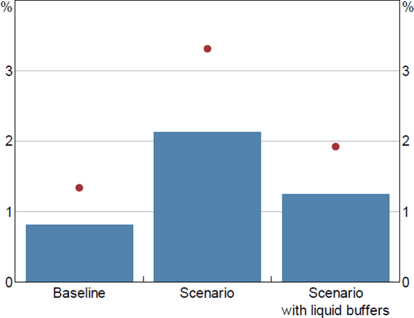
The macroeconomic scenario leads to household debt-at-risk as a share of housing debt increasing by only a small amount, from 0.8 per cent to 2.1 per cent (Figure 8).[29] Foreclosure costs account for about ½ percentage point of that increase. These estimates are low because housing loans account for the majority of household debt in Australia and these tend to be very well collateralised. Many high LVR loans in Australia are also covered by lenders mortgage insurance (LMI), which also reduces bank losses. Without LMI protection losses would be about 1 percentage point higher.[30] The debt-at-risk estimate is a little lower in magnitude to mortgages loss rates in recent stress tests by regulators in Australia, Canada, the United Kingdom and the United States. However, the estimate is substantially lower than actual loss rates in Ireland and the United States during the global financial crisis. This is mainly because Australian mortgages have low LVRs by international and historical standards. For example, less than 10 per cent of new Australian loans are written at LVRs above 90 per cent compared to close to 50 per cent of new loans in countries that experienced a boom-bust cycle during the financial crisis (Kelly, Le Blanc and Lydon 2019).
Note: Dot excludes protection from lenders mortgage insurance
Sources: ABS; Authors' calculations; Melbourne Institute
The losses are also low because debt tends to be held by households who are well placed to service it, consistent with previous research (particularly Bilston et al (2015)). Highly indebted households tend to have lower estimated probabilities of unemployment and higher incomes. This means they are less likely to experience income shocks that will reduce their ability to meet mortgage repayments.
It is possible that our results overstate the extent of debt-at-risk because of some simplifications in our approach. For example, debt-at-risk is considerably reduced if we assume households can draw down on their pool of liquid financial assets (such as offset accounts, deposits and equities) to avoid default.[31] Stress would also be further alleviated if lending rates fell.
When we incorporate these loan loss estimates into the RBA bank stress testing model (see RBA (2017) for more details of the model) banks remain above their capital conservation buffer of 8 per cent, even when assuming loans are not protected by LMI. Of course, household loans only comprise 40 per cent of banks' total assets. If we assume banks are also exposed to losses on banks' other portfolios (such as business loans, securities and other assets), equivalent in magnitude to recent APRA stress tests, banks' capital ratios fall to around the top of their capital conservation buffer. This suggests that the Australian banking system remains robust to losses stemming from rising household debt, largely because they participate in very little high LVR lending and are well capitalised. This result is consistent with past Australian stress tests and academic work (Bilston et al 2015; Rodgers 2015; Byres 2018; IMF 2019).
3.2 The Resilience of Household Consumption
Even when the banking system remains sound, high debt may still affect the sensitivity of the broader economy to shocks through its effect on the resilience of household consumption. There are two shocks that can cause consumption to decline: reduced income and reduced wealth.
The mechanics of the income channel are well established and understood: if a recession causes household income to fall, this reduces households' lifetime income and they curtail their consumption in response (Friedman 1957). This effect will be amplified if the fall in income is permanent, there is increased uncertainty about the future (Carroll 1992) or if a proportion of households are liquidity constrained (Kaplan and Violante 2014).
The wealth channel has considerable empirical support, but its theoretical foundation is still debated. Sinai and Souleles (2005) argue that there should be no (or limited) effect on consumption from changes in housing wealth because households are perfectly hedged against future housing price changes through their consumption of housing services. Others account for the empirical evidence of wealth effects by suggesting that this relationship is instead capturing the effect of changing expectations for future income or cycles in housing transaction volumes, both of which are correlated with wealth. However, Campbell and Cocco (2007) present evidence that is consistent with these wealth effects being due to more than just an omitted variable. In particular, they show that the positive consumption response to wealth from older home owners is not offset by a negative response from young renters, whose consumption seems to be impervious to changes in housing prices.
A growing body of research also shows that debt amplifies wealth effects, starting with Gertler and Bernanke's (1989) observation that collateral constraints are relaxed when house prices rise.[32] More recently, Guerrieri and Lorenzoni (2017) and Berger et al (2018) show theoretically that even households who are able to refinance might increase their precautionary savings in recognition of the risk that their borrowing constraint could bind in future. Consistent with this, Dynan and Edelberg (2013) show that indebted households in the United States reported a greater reduction in risk tolerance and a more pronounced jump in concerns about their ability to sustain spending than other households during the global financial crisis. And a large body of work, across a wide range of countries, has shown that the decline in consumption relative to wealth (that is, the MPCw) during the financial crisis of 2008–09 was larger for households that had higher initial leverage.[33] Baker (2018) and Athreya et al (2019) argue that at least some portion of this reflects that more highly indebted households tend to also be liquidity constrained, though this finding may be US-specific given the larger role that refinancing plays in the United States.[34]
Our approach differs from these papers in that we simulate a hypothetical stress test using a scenario that is more severe than that experienced by Australia during global financial crisis. To our knowledge, no other paper has taken such an approach. We do this because of our belief that the absence of very large shocks to Australian households in recent decades, combined with possible nonlinearities in the response of households to shocks, means that we cannot use empirical estimates of the potential pullback in consumption during severe stress. Because of this, we take estimates from past international research where large shocks have occurred (such as Mian et al (2013)) and use these to calibrate a model of consumption, rather than attempting to estimate the debt amplifier effect using Australian data. This helps us understand whether high and increasing debt could amplify aggregate falls in consumption during severe downturns.
Our stress test uses the same household-level database as in the preceding section and the same macroeconomic scenario as used in that section (Table 4). In order to estimate the effect on consumption, we need data on each household's income, debt, wealth and consumption. The SIH data, which were used in the preceding section, can be matched with the HES – the key survey of household consumption used to determine weights in the consumer price index – to allow a matching of income and wealth with spending. Combining these datasets results in a smaller sample of 10,046 households, but the sample remains representative of national aggregates (for income, wealth and expenditure) and there is no obvious selection bias as to which households from the SIH do not fill in the HES.[35]
An important consideration is whether households' consumption is affected by their superannuation (pension) assets. In calculating the change in wealth from the scenario, we assume that younger households are not sensitive to changes in their superannuation, given that it is many years before they will be able to access this wealth. Specifically, we assume that wealth sourced from superannuation is only included in households' assets if the household head is over 40 years old, and it is vested linearly until they are 60 years old.[36]
Our approach then involves calculating the change in consumption for each household, j:
where and are the respective changes in income and wealth from the stress scenario, and MPCY and MPCW are the marginal propensities to consume from income and wealth. This is then aggregated to get the change in economy-wide consumption. We also assume that households consume at least the amount given by the HEM used by banks when assessing loan serviceability, which accounts for the fact that some basic level of consumption is required for living. This acts to constrain the fall in consumption for a given household.
A central element of our stress test is the MPCs we assume for various households. As a baseline, we firstly consider a uniform scenario where all households have the same MPCs.
We benchmark the average MPCw of the population to 3 cents to the dollar based on past Australian studies. In particular, May, Nodari and Rees (2019) review the literature and find that elasticities are more stable through time than MPCs, and thus we construct our benchmark based on elasticities. We consider a housing wealth elasticity of approximately 0.16 and financial wealth of 0.12, consistent with the most recent estimates.[37] This leads to an MPC from housing wealth of 2.5 cents, an MPC from financial wealth of 5 cents and an overall MPCw of 3 cents. These are long-run estimates and are therefore consistent with a 2–3 year horizon.[38]
We benchmark the average MPCy to 55 cents to the dollar, based on May et al (2019). Estimates of MPCy in Australia vary widely, depending on methodology and whether it is based on macro or micro data. Our calibration is a little lower than Berger-Thomson, Chung and McKibbin (2009) which estimated MPCs of 0.6 to 1.0, but higher than other studies (Leigh 2012; Carroll et al 2017).
Having established a baseline, we then consider a scenario where we allow a correlation between MPCs and debt across households, while ensuring that the average MPC of the population is the same as in the baseline scenario. For this scenario, we calibrate the correlation between MPCs and debt based on previous research. For wealth, we assume a 100 basis point increase in leverage (debt relative to assets) leads to a 2 cent increase in the MPCw, based on Mian et al (2013). For income, we rely on Baker (2018) which finds a 100 basis point increase in the DTI ratio leads to a 6.2 cent increase in the MPCy.[39]
We consider other calibrations and extensions later on.
3.2.1 Uniform MPCs
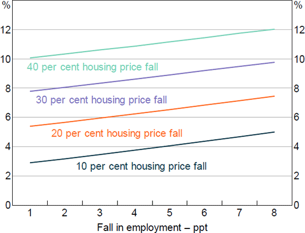
In the baseline stress scenario with uniform MPCs, there is a substantial fall in consumption of 12 per cent. Given the one-period nature of the framework, the change in consumption is best thought of as a 12 per cent peak-to-trough fall in real consumption per capita. Furthermore, the share of households consuming at the subsistence level increases from 13 per cent to 24 per cent when the shock is applied.[40] The scale of the shock in the scenario is somewhat arbitrary and so we also show the fall in consumption for a range of falls in employment and housing prices (Figure 9). This highlights that for the range of outcomes chosen, consumption is more sensitive to the fall in housing prices than the increase in unemployment.
The fall in consumption is much larger than those embodied in previous stress tests by APRA and the IMF in Australia which also involved severe recessions. It is also moderately larger than Ballantyne et al (2019), even when controlling for monetary stimulus. It is difficult to reconcile the differences, though it may reflect the uncertainty around modelling stress scenarios that are well out of the range of observed historical outcomes (including the presence of nonlinearities). We take comfort that these baseline results are not sensitive to the micro-simulation approach, since the wealth effects are a similar magnitude to those from back-of-the-envelope calculations using aggregate data from the ABS's Household Income and Wealth publication (ABS Cat No 6523.0).
Note: Other asset shocks adjusted commensurately to housing price adjustments
Sources: ABS; Authors' calculations; Melbourne Institute
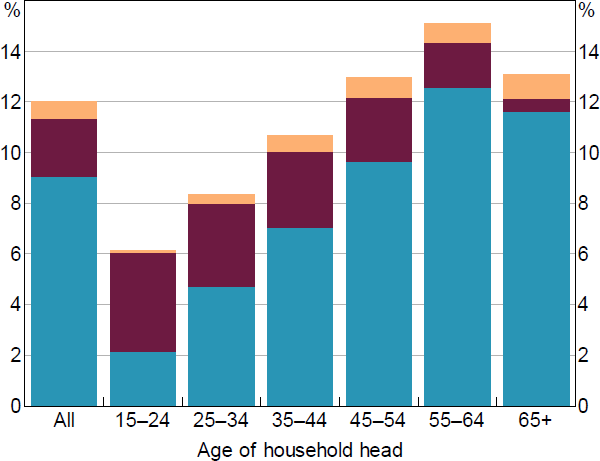
Roughly three-quarters of the consumption fall can be attributed to wealth effects, with the vast majority of this resulting from housing wealth (Figure 10). For households over 40 years old, about 20 per cent of the wealth effect is attributed to changes in superannuation assets. The rest of the fall in consumption is driven by income shocks. The fall in investment income, bonuses/overtime income and wage income are all of roughly equal magnitude.
It is interesting that the wealth effect in this model is larger than the income effect for any fall in housing prices greater than 10 per cent. This partly reflects that wealth shocks affect a larger share of the population (that is, any household with assets, compared to the income shocks which only affect workers who lose their job or receive variable income).[41] Thus, while unemployment, which is concentrated among a small subset of the population, tends to be a key driver of bank losses, it appears to be a less important driver for consumption in our stress scenario (at least in terms of its direct effect).
The model exhibits the expected effects across household types. For example, younger households are more sensitive to changes in income than in wealth, and this pattern reverses as households accumulate wealth. In the model, younger households are also more likely to become unemployed than older households, as expected.
Note: For uniform scenario where housing prices fall by 40 per cent and employment falls by 8 per cent
Sources: ABS; Authors' calculations; Melbourne Institute
3.2.2 MPCs correlated with debt
The focus of our consumption stress test is to see how different the estimated fall in consumption would be with MPCs that are positively correlated with household leverage or indebtedness. By design, this means that more leveraged households experience a larger fall in consumption than the baseline, and conversely that less leveraged households have a smaller fall (as seen in Mian et al (2013)). Critically, we ensure that the weighted average MPC stays the same as in the baseline scenario in order to focus on distributional effects rather than a general rise in MPCs.
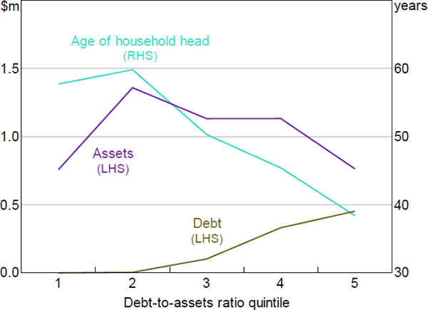
We find that aggregate wealth effects are slightly (but not meaningfully) smaller when MPCs are correlated with debt. The larger fall in consumption for highly leveraged households is more than offset by the smaller fall in consumption for lower leveraged households. A key reason for the overall result is that highly leveraged households tend to be less wealthy (have fewer assets) and younger (Figure 11). In contrast, lower leveraged households tend to be older households who have more assets and have been able to accumulate wealth and repay their debt over their lifetime.[42] The implication is that with MPCs increasing with leverage, the households that are most responsive to wealth shocks have little wealth to lose, while those experiencing the largest absolute falls in wealth are relatively insensitive to it.
Sources: ABS; Authors' calculations
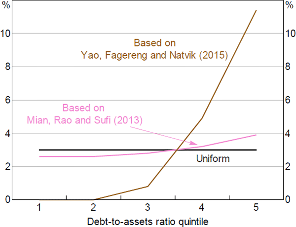
This point is illustrated more starkly when we increase the sensitivity of MPCs to leverage. Here we calibrate based on estimates from Yao, Fagereng and Natvik (2015) rather than Mian et al (2013). Using Norwegian data, they estimate that a 100 basis point increase in leverage leads to a 20 cent increase in the MPC from wealth, (compared to 2 cents in our original case). The MPCs calibrated from their results are shown in Figure 12. When we adopt this greater heterogeneity in our model, we find that wealth effects are smaller.[43] The overall fall in consumption is 11 per cent, compared to 12 per cent in the baseline. This is because the effect of the age dynamic outlined in Figure 11 becomes more pronounced in this specification – less leveraged households that tend to have higher assets see a smaller fall in consumption that more than offsets the larger falls by more leveraged households. This highlights that concentrating risks to a subset of the population tends to reduce the economy-wide effects on consumption.
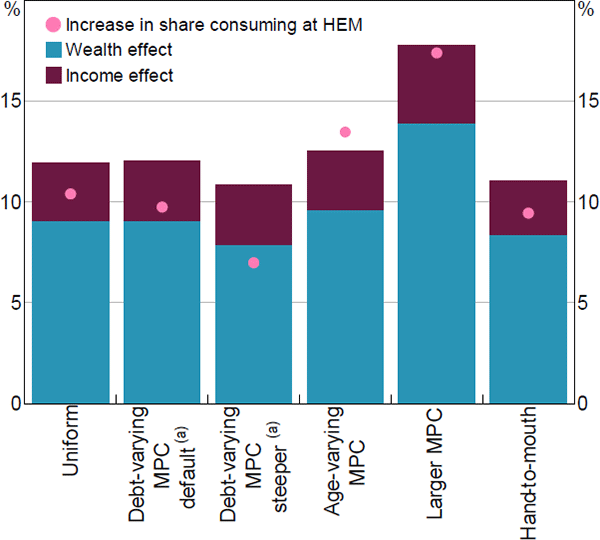
The remainder of this section considers three extensions to reconcile our findings with other work. We consider how our results change if MPCs vary with age, if households respond asymmetrically to negative shocks and if households are liquidity constrained. The results are shown in Figure 13. We then consider how the evolution of debt has changed the sensitivity over time.
Sources: ABS; Authors' calculations
Note: (a) ‘default’ based on Mian, Rao and Sufi (2013) and ‘steeper’ based on Yao, Fagereng and Natvik (2015)
Sources: ABS; Authors' calculations; Melbourne Institute
3.2.3 MPCw correlated with age
One key reason why assuming MPCs rise with leverage does not lead to a larger fall in aggregate consumption is because less leveraged households (who we assume have lower MPCs) tend to be older (i.e. retirees), with a larger stock of assets than highly leveraged households. However, several studies have found that the MPCw is typically higher for older households (Campbell and Cocco 2007; Calomiris, Longhofer and Miles 2012). To assess the implications of this, we allow MPCs to rise with household age and estimate the effect on consumption. It may be that older households (and, in particular, self-funded retirees) respond differently to changes in wealth than employed households, since their wealth is also their key source of income generation. In other words, self-funded retirees typically finance their spending through asset returns or by drawing down on their assets over time, rather than employment income. This may mean their consumption may be more sensitive to changes in their wealth, that is older households may actually have higher MPCs than those based on indebtedness from Mian et al (2013).
As before, we anchor the average MPC but vary the distribution of MPCs such that older households have higher MPCs. In this specification, the consumption fall is 12.5 per cent, which is moderately larger than the baseline scenario (‘Age-varying MPC’ column in Figure 13). Furthermore, the stress is potentially more pronounced than implied by the fall in consumption, because the share of households consuming at the subsistence level increases more markedly.
3.2.4 MPCs higher in downturns
Our estimates up to this point have been benchmarked to the economy-wide MPCs which are mostly estimated in periods of rising income and wealth. This may understate the effects if households are precautionary savers, households are constrained in taking on additional debt to smooth their consumption when the value of their collateral has fallen or if households exhibit loss aversion.[44] Indeed, there is evidence that households are more sensitive to falls in their wealth or income than to rises. Hviid and Kuchler (2017) and de Roiste et al (2019) find that the MPC from wealth is larger when wealth is falling than when it is rising, while Bunn et al (2018) and Christelis et al (2019) find the MPC from income is larger when income is falling.
With this in mind, we consider the effect of raising the average MPC from wealth from 3 cents to 5 cents and the MPC from income from 55 cents to 80 cents. This has a very large effect on our estimated fall in consumption, which rises to 17.8 per cent. The share of households consuming at the subsistence level also rises sharply (see ‘Larger MPC’ column in Figure 13).
3.2.5 Liquidity constraints
Other literature suggests that liquidity constraints (Kaplan, Violante and Weidner 2014; Baker 2018) or broader financial distress (Athreya et al 2019), rather than indebtedness per se, are what amplify consumption sensitivity to negative income shocks. We also find that indebtedness is positively correlated with measures of financial distress (such as ability to pay bills and seeking financial help), and, thus, our specification also partly captures the financial distress channel. However, to more directly investigate the importance of liquidity constraints, we consider the effect of assuming liquidity-constrained households have higher MPCy than unconstrained households. While the literature tends to focus on income shocks, we also consider the case where liquidity-constrained households have higher MPCw as well.
In particular, we follow the framework set out in Kaplan et al (2014) and extended by Price et al (2019). We firstly define hand-to-mouth households as households whose liquid wealth is less than half their income each pay period.[45] We then assume that hand-to-mouth households have an MPCy of 1 (or about twice as large as non-hand-to-mouth households), consistent with the findings in the United States.[46] We also assume the MPCw is twice as large for hand-to-mouth households, but this is more speculative given that these are not calibrated from past studies. As before, we ensure that the average MPCy and MPCw are anchored at 55 cents and 3 cents, respectively. In this specification, the fall in consumption is about ½ percentage point lower than in the baseline case (see ‘Hand-to-mouth’ column in Figure 13). This implies that liquidity constraints are not an important source of vulnerability in stress events like the one we consider.
3.2.6 Changes in sensitivity over the past decade or two
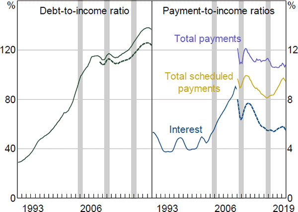
To investigate how the rise in indebtedness has affected the sensitivity of consumption to shocks, we compare results using data for 2003–04, 2009–10 and 2015–16. From 2003–04 to 2015–16, the aggregate household sector DTI ratio has increased by 30 percentage points, potentially signalling an increased vulnerability of the household sector to economic shocks. But an important factor contributing to some part of this rise has been lower interest rates, meaning that debt-servicing costs (the ratio of scheduled payments to total income) have remained relatively stable (at least between 2009–10 and 2015–16) as household indebtedness has risen (Figure 14). Moreover, household leverage has not risen noticeably due to strong growth in housing prices. It is therefore not clear that households have become more vulnerable (ignoring the potential for interest rates to rise from current levels).
The comparison uses data from the same surveys, the SIH and HES, at three points in time. We hold the elasticities of wealth and income constant, based on the assumption that these tend to be persistent through time. However, the MPCs will differ across time periods based on the underlying household data at the each point in time, in particular changes in consumption relative to wealth and income. Due to data limitations in the 2003–04 sample, we assume that bonuses and overtime income do not fall in the scenarios, and that the minimum consumption of households is the HPL (rather than the HEM).
Notes: Shaded areas indicate the sample periods for the 2003–04, 2009–10 and 2015–16 SIH data; dotted lines show net of offset balances
Sources: ABS; APRA; Authors' calculations
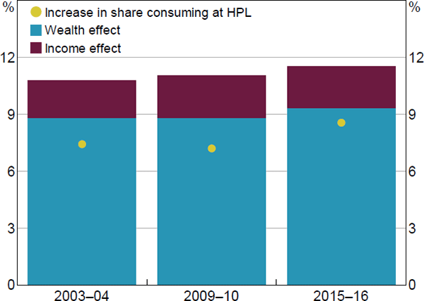
We find evidence that the vulnerability of household consumption has risen slightly over time. In particular, for the same macroeconomic shock, the fall in consumption is larger in 2015–16 (11.5 per cent) than in 2009–10 (11.0 per cent) and 2003–04 (10.8 per cent) (Figure 15).[47] The share of households consuming at subsistence levels after the shock increases more substantially over time. A bit less than half of the increased vulnerability from 2003–04 to 2015–16 can be attributed to greater household leverage. This increased leverage makes a given asset shock larger for the same household net wealth position. A similar-sized effect comes from a combination of households holding riskier assets and being more reliant on investment income over time. There is also a small effect from changes in the distribution of consumption spending. In particular, an increased share of total consumption now comes from higher-income households whose spending is less constrained by our assumption that minimum consumption will not fall below the poverty line.
Sources: ABS; Authors' calculations; Melbourne Institute
Footnotes
‘Severe but plausible’ scenarios are considered best practice in the stress testing literature (Borio, Drehmann and Tsatsaronis 2014). [22]
If job loss occurs, we assume individuals without children receive Newstart Allowance unemployment benefits (based on marital status), while parents receive the Parenting Payment. We calculate the change in disposable income by applying the shocks to gross income and then subtracting an estimate of income tax based on the relevant income tax tables. [23]
In practice, loans may enter arrears for many years before defaulting (Bergmann 2020); however, banks are required to provision for credit losses in a forward-looking way well before a borrower defaults. [24]
Bergmann (2020) finds that less than 10 per cent of arrears with an LVR below 90 per cent are foreclosed. [25]
If minimum mortgage repayments cannot be estimated because of inadequate data (or they are higher than current repayments), the household's current mortgage repayments are used. [26]
We also replicate our results using the Henderson Poverty Lines (HPL) published by the Melbourne Institute, which estimate the minimum income levels required to avoid a situation of poverty. The results were broadly similar, though the HPL is on average lower than the HEM. [27]
Loan losses may be higher if some households do not cut their consumption to these minimum levels and instead default earlier. [28]
The increase is slightly smaller than estimates in Bilston et al (2015) for earlier periods after accounting for the more severe scenario considered here. The results are smaller when we use the 2017–18 SIH sample. [29]
We assume an LMI payout ratio of 70 per cent, consistent with past APRA stress tests. Mortgage loans with an LVR that is currently above 80 per cent are assumed to have LMI. This likely understates LMI protection as it ignores repayments since origination. It is also possible that LMI providers may default during stress which would reduce this protection, though they tend to be well capitalised. [30]
About one-third of households with a negative financial margin have sufficient liquid assets to avoid default after two years. [31]
As an aside, the magnitude of this effect will vary across countries based on institutional features of credit markets. They are likely stronger in the United States than in Australia and other countries, due to the prevalence of long-term fixed-rate mortgage contracts. [32]
The initial paper in this strand of literature was Mian et al (2013), who used US data. Their results have since been replicated for Australia (Price et al 2019), Denmark (Andersen, Duus and Jensen 2016), Estonia (Kukk 2016), New Zealand (de Roiste et al 2019), Norway (Fagareng and Halvorsen 2016) and the United Kingdom (Bunn et al 2018). The main challenge to this strand of literature is Andersen et al (2016), which argues that the relationships between MPCw and leverage is driven by previous (one-off) purchases of consumer durables raising initial leverage, but then not being repeated in subsequent periods. [33]
For example, Price et al (2019) show that there is a ‘debt overhang’ effect in Australia even after controlling for liquidity constraints. [34]
The results on the banking stress test are robust to this smaller sample. [35]
Consumption effects are slightly larger if we relax this assumption, but the conclusions are unchanged. [36]
These are a little lower than estimates from before the financial crisis (Dvornak and Kohler 2003; Tan and Voss 2003). [37]
In existing Australian models, it typically takes two to three years for the majority of the effects to flow through to consumption (May et al 2019). [38]
Baker (2018) estimates elasticities rather than MPCs, but we adjust these by using the consumption-to-income ratio. [39]
The Poverty in Australia report (Davidson et al 2020) also finds that around 14 per cent of households live below the poverty line. [40]
The income effect may also be larger if individuals experience falls in hours worked or wage freezes, or if they reduce consumption due to uncertainty around their employment (even if they end up keeping their job). [41]
As an aside, while highly leveraged households tend to have lower assets, they tend to have higher incomes from which to service their debt. Thus, higher incomes at least partly offset the potential vulnerability of highly indebted individuals having less security on their loans. [42]
Hviid and Kuchler (2017) find a correlation between MPC and DTI ratios, rather than debt-to-asset ratios. When we assume their specification, the consumption fall (12½ per cent) is larger than the uniform scenario. [43]
Relatedly, several studies have found that in periods where housing prices are rising, the MPCw is higher for low-income households than high-income households because this reduces borrowing collateral constraints and enables them to raise consumption. When we calibrate this in the model, the overall effects tend to be lower because low-income households have less ability to reduce consumption. [44]
An important feature of this household type is that it includes liquidity-constrained households with large illiquid wealth, known as wealthy hand-to-mouth, because they face a trade-off in accessing their illiquid wealth and incurring costs to meet current consumption. We also account for mortgage prepayment buffers where available, though this does not materially affect the results. [45]
Price et al (2019) do not find evidence that hand-to-mouth households are more sensitive to changes in their income or home values than non-hand-to-mouth households, though the estimation period was not during a severe recession. However, La Cava, Hughson and Kaplan (2016) find hand-to-mouth households show a stronger propensity to consume out of cash flows than non-hand-to-mouth households. [46]
The fall in consumption is even smaller in 2009–10 (10.8 per cent) and 2003–04 (9.6 per cent) if we assume the MPCs are constant, rather than the elasticities. [47]