RDP 2019-07: MARTIN Has Its Place: A Macroeconometric Model of the Australian Economy 5. Model Dynamics
August 2019
- Download the Paper 1,572KB
In this section, we describe some of the dynamic properties of MARTIN. We first show the responses of key macroeconomic variables to three exogenous innovations, or shocks: an increase in the cash rate, a depreciation of the real exchange rate and a fall in housing prices. To provide some context for the results, we compare MARTIN's responses in the cash rate and exchange rate exercises to those from the RBA's DSGE model, MSM. We then compare the unconditional moments of some of MARTIN's key variables to their empirical counterparts.
5.1 An Increase in the Cash Rate
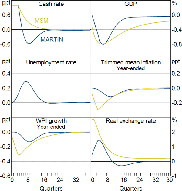
Figure 12 shows the responses of key aggregate variables to a 100 basis point increase in the cash rate that persists for four quarters, after which the cash rate follows its standard reaction function. The increase in the cash rate translates into higher mortgage and business lending rates, which raises borrowing costs for firms and households. It also leads to an appreciation of the real exchange rate. The net effect is to lower the level of GDP by around 0.8 per cent six quarters after the shock. The lower level of economic activity translates into an increase in the unemployment rate, which rises by 0.3 percentage points. The decline in aggregate demand and weaker labour market conditions contribute to a reduction in wages growth and inflation, which fall by a little less than 0.2 percentage points in year-ended terms after two years.
The GDP response to higher interest rates in MARTIN is similar to the response in MSM. However, the declines in wages growth and inflation in MARTIN are smaller than in MSM, and occur with a lag. In MSM, firms are forward looking and respond to the anticipated fall in demand after an increase in the cash rate by lowering their prices. In MARTIN, inflation does not decline until the contraction in demand translates into a rise in the unemployment rate and a fall in input costs.
Sources: Authors' calculations; RBA
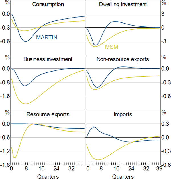
In common with other Australian macroeconomic models (Lawson and Rees 2008; Gibbs et al 2018), dwelling investment is the most interest-sensitive component of expenditure in MARTIN, declining by slightly more than three per cent following a 100 basis point increase in the cash rate (Figure 13). Household consumption declines by a bit less than GDP. However, because it accounts for a large share of expenditure, consumption makes a large contribution to the overall contraction in economy activity. The declines in consumption and dwelling investment in MSM are broadly similar to those in MARTIN, although MSM's responses are somewhat more persistent.
In MARTIN, business investment declines by about as much as GDP following an increase in interest rates. At first glance, the size of this response is somewhat surprising, as previous research has indicated that Australian firms' investment decisions are not sensitive to changes in interest rates (Lane and Rosewall 2015). It turns out that this is also the case in MARTIN; the direct response to increased funding costs accounts for only a quarter of the total decline in business investment. The rest of the investment response is due to lower aggregate demand, which reduces firms' incentives to invest. Funding costs play a larger role in determining investment in MSM, and in that model business investment declines by twice as much as in MARTIN.
Sources: Authors' calculations; RBA
The response of exports and imports to interest rates is a key difference between MARTIN and MSM. In MARTIN, non-resource exports decline by around 0.3 per cent following the increase in interest rates, while imports increase by around 0.25 per cent. Both responses are largely due to the appreciation of the real TWI, which reduces the international competitiveness of Australian-produced goods and services; the increase in imports is partly mitigated by the contraction in domestic demand. Although the response of non-resource exports volumes in the DSGE model is similar to the response in MARTIN, in MSM import volumes also decline.
The contrasting response of imports in the two models reflects differences in the speed of exchange rate pass-through. The relevant price for determining import volumes in MARTIN is the import price deflator. This captures ‘first-stage’ exchange rate pass-through (that is, the response of import prices at the docks to exchange rate changes). Exchange rate movements typically move the import price deflator one-for-one within a couple of quarters. Import volumes are estimated to be highly responsive to this relative price. In MSM, import volumes depend on ‘second-stage’ exchange rate pass-through (that is, the response of the prices faced by households and firms to changes in the exchange rate). Second-stage pass-through is generally estimated to occur slowly and to be incomplete (Chung et al 2011; Burstein and Gopinath 2014). Because of this, in MSM the income effect of lower aggregate demand overwhelms the price effect of the appreciation and import volumes decline. Better understanding the behaviour of import volumes following exchange rate movements would be a useful avenue for future research.
The response of resource exports also differs between the two models. In MARTIN, resource exports initially do not respond to the increase in interest rates because the productive capacity of the resources sector is unchanged in the short run. Over time, however, the appreciation of the Australian dollar means that some marginal investment in the resources sector does not occur. As a result, resource exports decline slightly after a few years. In MSM, resource firms can alter their production in the short run and so output falls immediately after a rise in interest rates.
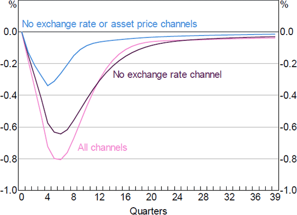
Figure 14 gives a sense of the relative contributions of the different channels of monetary transmission to the response of economic activity.[26] The line labelled ‘All channels’ replicates the response of GDP to the 100 basis point increase in the cash rate shown in Figure 12. In the line labelled ‘No exchange rate channel’ we impose the same interest rate path, but hold the real exchange rate fixed at its initial level. With this restriction, the level of GDP falls by around 0.6 per cent below its baseline level, compared to 0.8 per cent in the ‘All channels’ case. This indicates that the exchange rate channel accounts for around a quarter of the total effect of monetary policy on GDP. In the line labelled ‘No exchange rate or asset price channels’, we once again hold the exchange rate fixed and also turn off the response of housing and equity prices. In this case, the fall in GDP is close to 0.3 per cent, indicating that the asset pricing channel accounts for close to half of the overall GDP response to changes in interest rates. The remaining GDP response to interest rate changes reflects the other channels of monetary policy transmission, including the cash flow channel and the intertemporal substitution channel.
Sources: Authors' calculations; RBA
5.2 A Real Exchange Rate Depreciation
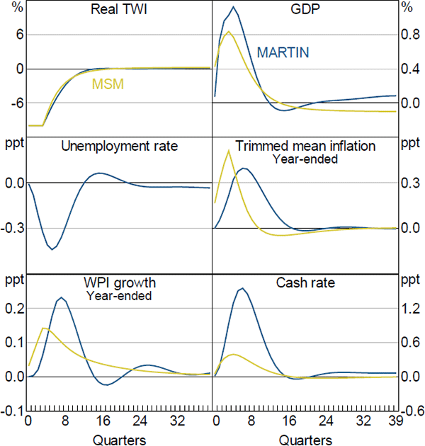
Figure 15 shows the responses of six key aggregate variables to a transitory 10 per cent real exchange rate depreciation. The depreciation reduces the price of Australian-produced goods and services relative to goods and services produced overseas. The resulting increase in demand for Australian goods and services raises the level of GDP by around 1 per cent after one to two years and lowers the unemployment rate by 0.4 percentage points. The expansion in economic activity and fall in the unemployment rate leads to an increase in wages growth. Increased wages growth and an increase in the price of imported goods and services raise firms' costs. In conjunction with the increase in demand, this leads to higher inflation, which rises by 0.3 percentage points. Higher inflation and a lower unemployment rate lead to an increase in the cash rate.
Sources: Authors' calculations; RBA
The responses of GDP, inflation and wages in MSM are all similar to those in MARTIN, although the pick-up in wages growth and inflation once again occur more quickly in MSM. The increase in the cash rate is also smaller in MSM. The differences in timing between the two sets of responses are in part due to the importance of expectations in MSM. Because households and firms in MSM are forward looking, they realise that the depreciation of the exchange rate will be inflationary and immediately adjust their wage demands and prices in response.
5.3 A Fall in Housing Prices
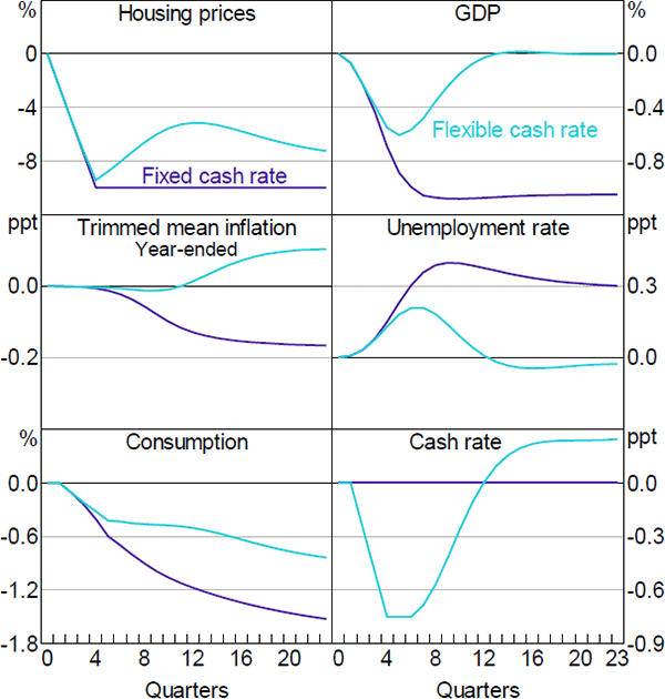
Figure 16 shows the responses of key aggregate variables to a persistent 10 per cent exogenous fall in housing prices. A decline in housing prices reduces the level of economic activity and inflation. In the absence of offsetting positive developments, the lower inflation and higher unemployment rate this implies could lead to a reduction in interest rates. To isolate the effects of lower housing prices from the effects of lower interest rates, we show two sets of results. In the first, we hold the cash rate fixed at its initial level. This shows the effects of lower housing prices independently of monetary policy. In the second, we impose an interest rate path that returns the level of economic activity to its previous trend after two to three years.
Sources: Authors' calculations; RBA
Lower housing prices affect the economy in several ways. Because housing is the largest component of household assets, lower housing prices reduce household net wealth, which lowers consumption. Lower housing prices also make new home building less profitable, which reduces dwelling investment. The decline in consumption and dwelling investment lowers aggregate demand, which reduces the incentives for firms to invest. The net effect, absent an interest rate response, is to lower the level of GDP by a bit more than 1 per cent below its baseline level after one to two years. The decline in economic activity reduces the demand for labour and causes the unemployment rate to increase by around 0.4 percentage points. The decline in economic activity and the higher unemployment rate leads to a fall in inflation of around 0.2 percentage points in year-ended terms.
The implications of lower housing prices are considerably smaller if monetary policy responds. The model's endogenous reaction function delivers a relatively slow interest rate response because it takes several quarters for inflation and the unemployment rate to respond to the fall in housing prices. However, because changes in housing prices are readily observable and strongly persistent, making the macroeconomic consequences predictable, this delayed response strikes us as unrealistic.[27] Therefore, the particular cash rate path that we consider involves a 75 basis point reduction in interest rates over four quarters following the decline in housing prices, after which monetary policy follows its standard reaction function.[28] This cash rate profile roughly halves the peak effect of lower housing prices on GDP and the unemployment rate, and returns these variables to their baseline trends within three years.
The reduction in the cash rate also raises housing prices relative to the scenario with a fixed cash rate. However, housing prices remain well below their initial level. This reflects the fact that monetary policy targets inflation and full employment, not asset prices. By limiting the decline in housing prices, monetary policy helps to support the level of economic activity. But other channels, such as the exchange rate channel and the intertemporal substitution channel are also at work. In practice, much of the recovery in GDP reflects an increase in export volumes and decrease in imports; even with a lower cash rate the level of consumption remains considerably below its baseline level following a persistent fall in housing prices.
5.4 Unconditional Moments
Another way to test the model's properties is to examine how well it can replicate key empirical features of the data, such as the means and standard deviations of macroeconomic variables. To calculate these moments in MARTIN, we run a large number of simulations. In each simulation we draw a selection of the reduced form residuals from the model's equations and impose these residuals on the model. We use a block bootstrap to draw the model residuals, which preserves the cross-variable and across-time correlation structure of the residuals observed in the data. After each simulation, we calculate the means and standard deviations of the model variables. Repeating this process for a large number of simulations gives us an indication of the unconditional moments of variables in the model.
Table 2 compares the unconditional means and standard deviations of selected variables in MARTIN to those in the data.[29] In most cases, the standard deviations of the variables in MARTIN are close to those in the data. One exception is GDP growth; its standard deviation in MARTIN is larger than its value in the data. This largely reflects that GDP in MARTIN is calculated as GDP(E), where the components of expenditure are added together. Empirically, GDP(E) growth has a larger standard deviation than GDP(A) growth – which is calculated as an average of expenditure, income and production measures and is the measure shown in the table. The standard deviation of GDP(E) is closer to the standard deviation of GDP growth in MARTIN.
| MARTIN | Data (1998–2018) | ||||
|---|---|---|---|---|---|
| Mean | Standard deviation | Mean(a) | Standard deviation | ||
| GDP growth | 2.8 | 1.6 | 3.1 | 1.0 | |
| Consumption growth | 2.8 | 1.3 | 3.4 | 1.4 | |
| Unemployment rate | 4.5 | 0.6 | 5.7 | 0.8 | |
| Trimmed mean inflation | 2.6 | 0.7 | 2.6 | 0.7 | |
| Headline inflation | 2.6 | 0.9 | 2.4 | 0.8 | |
|
Sources: ABS; Authors' calculations |
|||||
The means of the model's nominal variables are generally close to their empirical counterparts. The RBA has been broadly successful in meeting its inflation target over recent decades and this pins down the long-run means of these variables in MARTIN. The means of many of the activity variables in the data are larger than those in MARTIN. This likely reflects the lower potential output growth estimate in MARTIN compared to historical growth rates.
Footnotes
See Atkin and La Cava (2017) for a discussion of the channels of monetary policy in Australia. [26]
In contrast, a slower monetary response to the exchange rate movement described above is more plausible because exchange rates are volatile, meaning that it may be more reasonable to wait to assess the macroeconomic consequences of an exchange rate move before adjusting the cash rate. [27]
We calibrate the policy response by applying the policy rule's recommended reduction in interest rates – 75 basis points – contemporaneously with the fall in housing prices. [28]
We restrict our data sample to the period 1998–2018 as this corresponds to the sample for which we have a balanced panel of data in MARTIN. [29]