RDP 2019-07: MARTIN Has Its Place: A Macroeconometric Model of the Australian Economy 4. Core Equations
August 2019
- Download the Paper 1,572KB
In this section we describe the core behavioural equations in MARTIN. Our goal here is not to provide a comprehensive account of the full set of equations and identities, or the econometric details of the individual equations, all of which we provide in our online appendix. Rather, it is to highlight the economic intuition behind the key relationships that drive MARTIN's forecasts and scenarios.
In line with this goal, there are a number of small differences between the way in which we present individual equations in this section and the way in which they appear in MARTIN's code. One relates to the equations that take an error correction form. In describing these equations in the text, we make an explicit distinction between the long-run and short-run components. In practice, however, we estimate almost all of these equations using a one-step approach – that is, we estimate the short-run and long-run parts of the equations simultaneously. In addition, to simplify the presentation of the equations we omit terms that have no economic interpretation, such as dummy variables used to account for outlying observations.
Table 1 defines the variables used in the equations described below. To simplify notation, in the equations below we use capital letters to denote the level of a variable and lower case letters stand for the natural logarithm of a variable. The symbol refers to the quarterly change in the value of a variable. In all the ECM equations, the symbol is the speed of adjustment parameter and errort refers to the equilibrium error. The data used are quarterly. The estimation samples differ between equations. For most of the model's expenditure and labour market variables, such as consumption and the unemployment rate, our estimation samples begin in the 1980s or earlier. Using longer samples that include periods of heightened macroeconomic volatility helps us to pin down macroeconomic relationships that are harder to identify in the more stable economic environment that has existed since the early 1990s. In contrast, we estimate the equations of most of the nominal variables, including inflation and wages growth, over samples starting in the 1990s. This reflects structural breaks in many of these series that occurred around this time, which makes estimation over longer samples unreliable.[11]
| Variable | Definition | Specification | Value | Source |
|---|---|---|---|---|
| Trend and supply side | ||||
| pi_e | Inflation expectations | Per cent | RBA | |
| RSTAR | Neutral interest rate | Per cent | Real | RBA |
| ta | Trend labour productivity | Log | Real | RBA |
| thpp | Trend average hours worked | Log | RBA | |
| TLUR | NAIRU | Per cent | RBA | |
| tpop | Trend population | Log | RBA | |
| ty | Trend growth (for Okun's Law) | Log | Real | RBA |
| Household sector | ||||
| hcoe | Compensation of employees | Log | Real | ABS, RBA |
| hdy | Household disposable income | Log | Real | ABS, RBA |
| hnw | Household net wealth | Log | Real | ABS, RBA |
| hoy | Household non-labour disposable income | Log | Real | ABS, RBA |
| nhc | Household credit | Log | Nominal | ABS, APRA, RBA |
| nhfa | Household financial assets | Log | Nominal | ABS |
| rc | Household consumption | Log | Real | ABS |
| Housing sector | ||||
| id | Dwelling investment | Log | Real | ABS |
| kid | Dwelling stock | Log | Real | ABS, RBA |
| otc | Ownership transfer costs | Log | Real | ABS |
| ph | Housing prices | Log | Nominal | Corelogic, RBA |
| prt | Household rents | Log | Nominal | ABS |
| rph | Housing prices | Log | Real | ABS, Corelogic, RBA |
| Business sector | ||||
| IBCR | Cost of capital | Per cent | RBA | |
| ibn | Non-mining business investment | Log | Real | ABS |
| IBNDR | Non-mining depreciation rate | Per cent | ABS, RBA | |
| ibre | Mining investment | Log | Real | ABS |
| IBREDR | Mining depreciation rate | Per cent | ABS, RBA | |
| kibre | Mining capital stock | Log | Real | ABS |
| nibre | Nominal mining investment | Log | Nominal | ABS |
| Foreign trade and foreign sector | ||||
| m | Imports | Log | Real | ABS |
| tot | Terms of trade | Log | ABS | |
| xre | Resource exports | Log | Real | ABS |
| xs | Services exports | Log | Real | ABS |
| wy | Major trading partner GDP | Log | Real | RBA |
| Prices and labour market | ||||
| le | Employment | Log | ABS | |
| LUR | Unemployment rate | Per cent | ABS | |
| nulc | Nominal unit labour costs | Log | Nominal | ABS |
| nulcbs | Nominal unit labour costs with Balassa-Samuelson adjustment | Log | Nominal | ABS, RBA |
| p | Consumer price index | Log | Nominal | ABS |
| Prices and labour market | ||||
| pae | Average earnings from the national accounts | Log | Nominal | ABS, RBA |
| pex | Headline CPI excluding volatile items | Log | Nominal | ABS |
| poil | Oil price in Australian dollars | Log | Nominal | Bloomberg, RBA |
| ptm | Trimmed mean inflation | Log | ABS | |
| pw | Wage price index, excluding bonuses | Log | Nominal | ABS |
| rlc | Labour costs (average hourly earnings) | Log | Real | ABS |
| rulc | Real unit labour costs | Log | Real | ABS |
| Financial markets | ||||
| N2R | Two-year government bond rate | Per cent | Nominal | RBA, Yieldbroker |
| NBR | Business lending rate | Per cent | Nominal | RBA |
| NBRSP | Business spread to cash rate | Percentage points | Nominal | RBA |
| NCR | Overnight cash rate | Per cent | Nominal | RBA |
| NMR | Mortgage rate | Per cent | Nominal | RBA |
| NMRSP | Mortgage rate spread to cash rate | Percentage points | Nominal | RBA |
| peqi | Market price of equities | Log | Nominal | Bloomberg, MSCI, RBA, Refinitiv |
| RCR | Cash rate | Per cent | Real | RBA |
| rewi | Export-weighted exchange rate index | Log | Real | BIS, RBA |
| RMR | Mortgage rate | Per cent | Real | RBA |
| rtwi | Trade-weighted exchange rate index | Log | Real | RBA |
| WR2SP | Spread from Australian to G3 policy rates | Percentage points | Real | RBA |
| WR2SP_AVE | Average WR2SP since 1993 | Percentage points | Real | RBA |
| National aggregates | ||||
| AT | Net asset transfers between household and public sectors | Level | Real | RBA |
| g | Public demand | Log | Real | ABS |
| gne | Gross national expenditure | Log | Real | ABS |
| iad | Import-adjusted demand | Log | Real | RBA |
| ny | Gross domestic product | Log | Nominal | ABS |
| SD | Statistical discrepancy | Level | Real | ABS |
| V | Change in inventories | Level | Real | ABS |
| y | Gross domestic product | Log | Real | ABS |
| Implicit price deflators (IPD) | ||||
| pc | Household consumption IPD | Log | ABS | |
| pdfd | Domestic final demand IPD | Log | ABS | |
| pgne | Gross national expenditure IPD | Log | ABS | |
| pibn | Non-mining business investment IPD | Log | RBA | |
| pibre | Mining business investment IPD | Log | RBA | |
| pid | Dwelling investment IPD | Log | ABS | |
| pm | Imports IPD | Log | ABS | |
| pmcg | Imported consumption goods IPD | Log | ABS | |
| pxre | Resource exports IPD | Log | ABS | |
| py | Gross domestic product IPD | Log | ABS | |
4.1 The Supply Side
The supply side of the model consists of exogenous processes governing the evolution of trend labour productivity growth, trend population growth and trend average hours worked.[12] Together, these variables determine the potential growth rates of GDP, employment and real wages.
The log of trend labour productivity, tat, follows a random walk with drift, . The drift term is an AR(1) process that mean-reverts at a 5 per cent quarterly rate:
where is the long-run mean of labour productivity growth. We restrict the coefficient on the lag of the drift term to equal 0.95. This ensures that the drift term accounts for persistent variation in productivity growth, while still having a well-defined mean. An alternative would be to allow trend productivity growth to follow a random walk (by setting the coefficient on lagged productivity growth equal to one). In practice, this would produce similar estimates of trend productivity growth over history. However, it would make the model unstable in simulations because productivity growth could increase or decrease without bound.
The log of trend population, tpopt, also follows a random walk with drift, . The drift term is an AR(1) process that mean-reverts at a 5 per cent quarterly rate:
where is the long-run mean of population growth.
The log of trend average hours worked, thppt, follows a random walk with drift, . Unlike productivity and population growth, we restrict the long-run drift of hours worked to converge to a mean of zero at a 5 per cent quarterly rate. This ensures that in long-run projections the decline in hours worked observed over recent decades eventually comes to an end.
In the current version of MARTIN, we set long-run annual labour productivity growth to 1.5 per cent and long-run annual population growth to 1.25 per cent, meaning that the economy's long-run potential growth rate is 2.75 per cent.
Because aggregate supply ultimately determines the growth rates of income and expenditure, the supply-side trends enter many of the equations in MARTIN. As such, we need to derive values for these variables over history. To do so, we assume that the measured values of labour productivity, population and hours worked in the data equal their long-run trends plus a random error term, estimate the parameters of the models via maximum likelihood, and then conditional on those parameter estimates use a Kalman filter to infer the value of the long-run trends given the data. In estimation we restrict the standard deviation of the error in the drift terms to be 1 per cent of the standard deviation of the errors in the level equations. This ensures that the drift terms capture low frequency changes in the value of these series without overfitting the data.
Figure 2 plots the estimated trends and the economy's implied potential growth rate in annualised terms. Trend population growth averaged around 1¾ per cent in the 1980s and 2010s, and around 1½ per cent between those times. Trend labour productivity growth declined during the 1980s, increased during the 1990s and has since settled at around 1¼ per cent. The decline in average hours worked has made a small subtraction from potential growth over recent decades. Summing these trends together, we estimate that potential GDP growth averaged a bit over 3 per cent between the early 1980s and early 2000s and has declined slightly to around 2¾ per cent since then.
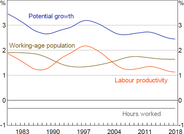
Sources: ABS; Authors' calculations; RBA
4.2 Consumption and the Household Sector
4.2.1 Consumption and household income
The consumption equation captures the spending and saving decisions of households. We model consumption within a permanent income hypothesis framework, which implies a long-run relationship between consumption, household income and net wealth (Figure 3).[13] This relationship can also be motivated as the linearisation of the household sector's budget constraint (Lettau and Ludvigson 2001). To ensure that consumption grows at the same rate as income and net wealth along a balanced growth path, we restrict the coefficients on these variables to sum to one. We also include the real interest rate in the long run part of the equation to capture the idea that it is optimal for households to save a larger proportion of their income when real interest rates are high. We impose a small coefficient on this latter variable, which implies that a 100 basis point decrease in interest rates raises the long-run level of consumption by 0.05 per cent. We also include a level shift in the long-run equation that occurs in 2007:Q1. This captures an observed shift in the household saving rate, conditional on the levels of income and wealth, which occurred at this time.
Consumption deviates from its long-run equilibrium due to short-run movements in labour and non-labour income and net wealth. Along a balanced growth path, the economy's trend growth rate (which is the sum of trend labour productivity growth, population growth and growth in hours worked) also influences consumption. In this way, the equation allows for the possibility that some households make their consumption decisions based on long-run income expectations while the expenditure of other households, possibly because they face collateral or liquidity constraints, is more sensitive to current income. Because the model's estimates of trend labour productivity and population growth are time-varying, the equation should be robust to changes in trend growth over time. We also include the change in the unemployment rate to capture the precautionary savings motive induced by economic uncertainty, as well as to account for the possibility that changes in the unemployment rate alter the distribution of income, and hence consumption, in ways that aggregate household income does not capture (Muellbauer and Williams 2011).
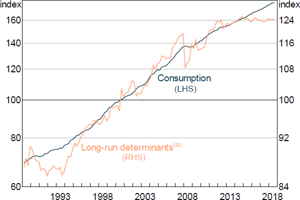
Note: (a) Includes household income, net wealth and the cash rate
Sources: ABS; Authors' calculations
4.2.2 Household balance sheet
The net wealth of households is made up of their assets less their liabilities. We model each of these quantities in nominal terms. Household assets consist of non-financial and financial assets. The growth rate of non-financial assets is linked to the growth rate of the value of the housing stock, that is, housing prices times the housing stock. We model the housing stock using a standard capital accumulation equation in which next quarter's housings stock equals the undepreciated component of this quarter's housing stock plus gross dwelling investment. The housing price and dwelling investment models are described in Section 4.3.
The equation for household financial assets assumes that households hold a constant proportion of their portfolio in risky assets (Merton 1969).[14] This leads to an error correction specification where financial assets and equity values move together in the long run:
To ensure a stable long-run ratio between financial assets and equity values, we restrict the coefficient on equity values to equal one. In the short run, trend real growth and movements in equity prices also influence financial assets. We model equity values as expected earnings for listed firms divided by the earnings yield. Expected earnings depend largely on aggregate profits and commodity prices, while the earnings yield is related to the gap between the required rate of return on equities (proxied by the business lending rate) and the economy's trend growth rate.
The household sector's liabilities consist of liabilities to the financial sector (that is, household credit) and household debt outside the Australian banking system. In the long run, the stock of household credit is determined by the value of housing assets and the average loan-to-valuation ratio of housing loans. We proxy for the latter with the real mortgage interest rate, which captures the tendency for loan-to-valuation ratios to increase when real mortgage rates decline.
In the short run, the growth rate of nominal household credit depends on housing price growth, growth in the dwelling stock, changes in mortgage interest rates and the rate of inflation. The coefficient restrictions ensure that the stock of credit grows at the same rate as nominal GDP along the model's balanced growth path.
Household debt outside the banking system is a volatile series and hard to account for using standard macroeconomic data. Because of this, we model this component of liabilities as an autoregressive process, constraining its mean growth to equal the rate of trend nominal GDP growth along a balanced growth path.
4.3 The Housing Sector
The dwelling investment, housing price and rents equations capture the demand for and supply of housing services. The behavioural dynamics underlying these equations reflect households' decisions about whether to buy, sell or build dwellings.
4.3.1 Dwelling investment
We model dwelling investment using an ECM with consumption, real mortgage interest rates and the relative price of dwelling investment. In the long run, households are assumed to allocate a stable share of their expenditure to housing and non-housing consumption, conditional on the level of interest rates. This implies that the ratio of nominal dwelling investment to nominal consumption expenditure will fluctuate around a constant mean, which is strongly evident in the data (Figure 4). A decrease in real interest rates lowers the cost of borrowing to construct new housing as well as the cost of new housing relative to established housing (whose price tends to rise with lower interest rates). This makes dwelling investment more profitable and raises its expenditure share relative to consumption.
Dwelling investment can deviate from its long-run equilibrium because of short-run movements in the nominal mortgage interest rate and real housing prices. Along a balanced growth path, real dwelling investment grows at the economy's trend growth rate.
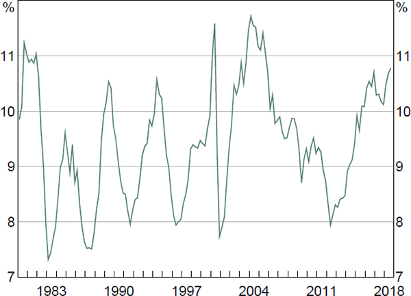
Sources: ABS; RBA
4.3.2 Housing prices
We model housing prices using an ECM similar to that in Fox and Tulip (2014). Housing prices are expected to tend towards their fundamental value, which is the price where households are indifferent between owning and renting. We assume that variation in the user cost of owning a home is driven by movements in the real mortgage interest rate.[15] In the long run, if the real mortgage rate is constant, nominal housing prices will grow in line with rents. Like Fox and Tulip, we find that the rents–user cost framework can account for much of the growth in housing prices over recent decades (Figure 5).
In the short run, changes in housing prices have a large inertial component, and are also influenced by recent movements in nominal mortgage interest rates.
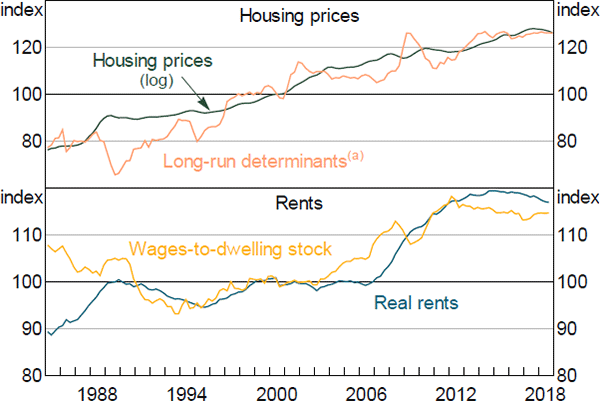
Note: (a) Includes CPI rents and the real cash rate
Sources: ABS; Authors' calculations; Corelogic
4.3.3 Rents
In the long run, real rents depend on the demand for and supply of housing. We measure the demand for housing using real compensation of employees – the wage component of real household income. The supply of housing is given by the housing stock. This relationship can account for a large part of the low frequency movement in rents over recent decades (Figure 5). Because rent inflation is a highly persistent series, much of its short run behaviour is accounted for by its own lag.
4.4 Business Investment
We model non-mining and mining investment separately, reflecting the fact that the determinants and historical behaviour of these two series differ substantially.
4.4.1 Non-mining business investment
The long run component of the non-mining business investment equation is based on neoclassical investment theory, which asserts that firms invest to the point where the marginal return on an additional unit of capital is equal to its user cost (Jorgenson 1963). In MARTIN, this is captured by a long-run relationship between investment, output and the cost of capital. We use gross national expenditure (GNE) as our measure of output, rather than GDP, because it abstracts from large movements in resource export volumes, which are unlikely to create demand for non-mining investment. However, we include the mining investment share of GDP as an additional variable to capture the tendency for expansions in the resources sector to draw resources away from other parts of the economy. In most theoretical models, the steady-state investment-to-output ratio is a function of trend GDP growth and the capital depreciation rate. Therefore, we also include these variables in the equation.
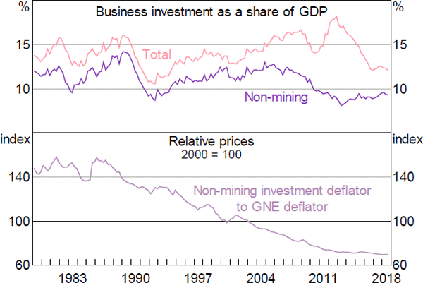
Any empirical investment equation using Australian data must reconcile three stylised facts: (i) the ratio of nominal business investment to GDP has had a reasonably stable mean over recent decades; (ii) the relative price of business investment (which is a component of the cost of capital) has declined substantially over this time; and (iii) most time series estimates suggest that the direct response of investment to changes in interest rates (another component of the cost of capital) is small (Figure 6). To account for these features of the data, we separate the relative price of non-mining business investment from other components of the cost of capital and impose a coefficient of −1 on the former.[16] This coefficient restriction means that changes in the relative price of investment goods do not alter the investment share of GDP in the long run. We calibrate the coefficient on the other components of the cost of capital to equal –0.4, which is consistent with a range of overseas and Australian evidence (Antràs 2004; Cockerell and Pennings 2007), as well as with the coefficient on real wages in MARTIN's employment equation.[17]
Quarterly changes in non-mining business investment are volatile and hard to explain using macroeconomic data. Reflecting this, the short run component of the equation is parsimonious, only including the two-quarter change in GNE.
Sources: ABS; Authors' calculations
4.4.2 Mining investment
Resource firms produce undifferentiated products and take the prices of these products as given. These prices (equal to the world price of resources, adjusted for the value of the Australian dollar exchange rate), relative to the prices of non-resource goods and services, dictate the size of the resources sector. A rise in resource export prices increases the size of the resources sector, and hence the mining investment share of GDP. Holding relative resource export prices fixed, this share converges to a stable value in the long run, which depends on the economy's trend growth rate as well as the depreciation rate of capital in the resources sector. In the short run, the growth rate of resource exports depends positively on recent changes in relative resource export prices and the economy's trend growth rate.
4.5 Foreign Trade
We disaggregate exports into five categories – services, manufactures, agricultural, resources and other – reflecting the different determinants and trends in these series. In contrast, we model imports at the aggregate level.
4.5.1 Non-resource exports
The non-resource exports equations share a common structure. In the long run, each component of exports depends on overseas demand, measured as the export-weighted GDP of Australia's major trading partners, and relative prices, measured as the real export-weighted exchange rate. An increase in overseas demand raises export volumes, whereas an increase in the relative price of goods and services produced in Australia lowers exports. We constrain the demand elasticities to equal one, but estimate the price elasticities. The price elasticities turn out to differ substantially between export components.
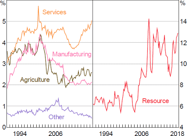
Global trade liberalisation, lower transport costs and other related developments have led to substantial changes in the ratio of exports to GDP over the past thirty years that cannot be fully accounted for by growth in foreign GDP or changes in relative prices. These shifts in trade shares are particularly evident in exports of services and manufacturing products (Figure 7). To account for these features of the data, we include time-varying constants in the manufactured and services exports equations. We estimate these constants using state-space methods.[18] In the short run, growth in exports generally depends on growth in foreign demand and changes in relative prices.
For example, the equation for services exports is:
Time-varying constant:
As the equations for the remaining categories of non-resource exports are similar to that of services exports, we leave the precise specifications of these equations to the Online Appendix.
Sources: ABS; RBA
4.5.2 Resource exports
In the long run, resource exports are determined by the supply of mining output. We assume that mining supply is proportional to the capital stock of the resources sector, reflecting the fact that production of mining commodities is highly capital intensive. Mining capital affects exports with a lag, because there is often a delay between the installation of new capital and the time when it starts to produce output.
Resource exports volumes vary considerably from quarter to quarter, often because of supply shocks that temporarily reduce output, as well as the lumpy nature of new production. Because of this, the coefficient on lags of resource exports is negative – a decrease in resource exports growth in one quarter is likely to be partially unwound in the subsequent quarter.
4.5.3 Imports
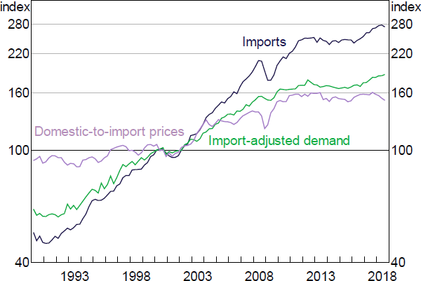
In the long run, import volumes depend on the level of domestic demand and the relative price between imports and goods and services produced in Australia (Figure 8). We use an import-adjusted measure of demand that weights each component of domestic final demand by its relative import intensity.[19] So, for example, an increase in business investment – which is relatively import intensive – will cause a larger increase in imports than a similar-sized increase in dwelling investment – which has a low import intensity. The relative prices term is the ratio of the import price deflator to the domestic final demand deflator. The estimated coefficient on this term is close to –1. This is consistent with the fact that the ratio of nominal import values to nominal GDP has been broadly stable over the estimation sample. However, it has the implication that import volumes respond quickly to exchange rate movements, which seems at odds with the observation that exchange rate pass-through to domestic prices occurs with a significant delay (Chung, Kohler and Lewis 2011). To reconcile these two stylised facts, we include the average of four lags of relative import prices in the long run part of the equation. This limits the speed with which changes in import prices translate into import volumes, and also prevents temporary exchange rate movements from driving large changes in imports. The long-run properties of the model, however, are unaffected by this modelling choice. In the short run, imports growth is a function of contemporaneous and lagged demand and relative prices.
Sources: ABS; Authors' calculations
4.6 National Accounts Aggregates
We construct the national accounts aggregates – gross domestic product, gross national expenditure and domestic final demand – by summing the expenditure components described above. For nominal values this summation exactly matches the published aggregates. But for the chain volume expenditure components, the summation only approximates to the published aggregates when relative prices change. In practice, these approximation errors are typically small, particularly for forecasts and scenarios constructed close to the national accounts reference year. Although more complex aggregation methods are possible, we found that simple aggregation introduces less bias in the forecasting process than these alternative approaches.
4.7 Prices and Wages
The prices and wages block of the model links the real and nominal sides of the economy. Developments in this block have a large influence on monetary policy settings and feed back into other aspects of the model, such as household income.
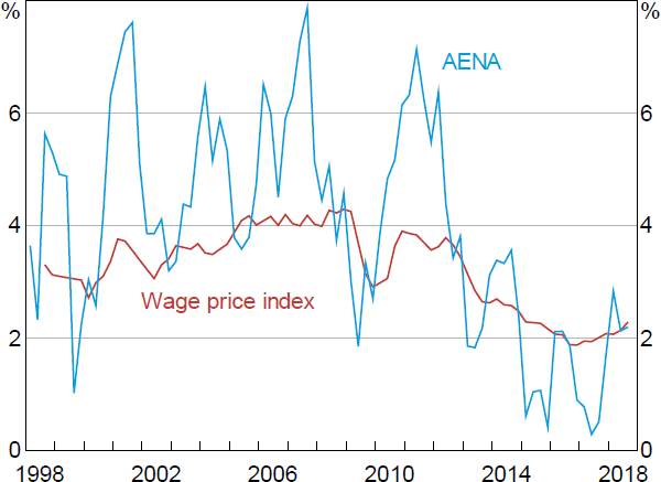
There are two main equations in the prices and wages block. The first is the equation for the wage price index (WPI). The WPI captures pure wage effects, abstracting from compositional changes in employment and labour quality. We map the WPI into average earnings from the national accounts (AENA), which incorporates compositional shifts and changes in labour quality and is the relevant wage measure for the determination of household income and prices (Figure 9). In turn, AENA feeds into nominal unit labour costs, and then into prices through the trimmed mean inflation equation, which is the second main equation in the prices and wages block.
Sources: ABS; RBA
Many of MARTIN's price and wage variables are influenced by the NAIRU and inflation expectations. Both of these variables are exogenous in the model and, as neither can be observed directly, are instead constructed using the approach described in Cusbert (2017).
4.7.1 Wage price index
We model the WPI using a Phillips curve approach. Less spare capacity in the labour market, as measured by a decreasing unemployment rate and smaller unemployment gap, will lead to faster wages growth. Higher inflation expectations and faster growth in the GDP deflator also raise wages growth, as nominal wages will need to increase more quickly to maintain a given real wage. An increase in productivity growth also leads to faster wage growth, because it raises the marginal product of labour.
Along a balanced growth path, the unemployment rate will converge to the NAIRU and inflation expectations and growth in the GDP deflator will converge to 2.5 per cent. When this occurs, growth in the WPI will reflect two factors: prices growth of 2.5 per cent; and real WPI growth, which will be proportional to labour productivity growth. However, real WPI will grow more slowly than aggregate labour productivity, because the WPI is partly quality adjusted.
4.7.2 Average earnings from the national accounts (AENA)
We map the WPI into AENA using the following equation:
Faster growth in the WPI feeds through to AENA. The pass-through is greater than one-for-one, because AENA tends to be more cyclical than the WPI. Along a balanced growth path, AENA grows at the sum of labour productivity growth plus inflation.
4.7.3 Trimmed mean inflation
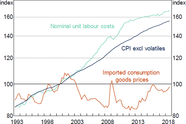
We model trimmed mean inflation using a mark-up model, similar to the specification described in Norman and Richards (2012). In the long run, firms are assumed to set their prices as a fixed mark-up over their input costs. As such, there is a long-run relationship between the price level, nominal unit labour costs and the price of imported consumption goods (Figure 10).[20] If prices are unusually low relative to input costs, we should expect inflation to be higher than usual as firms seek to restore mark-ups to their desired level. Similarly, if prices are unusually high relative to input costs, we should expect inflation to be lower than usual.
Sources: ABS; RBA
We restrict the coefficients on unit labour costs and import prices to sum to one. This condition, known as static homogeneity, ensures that the model has the desirable steady-state property that if all input costs were to double, consumer prices would also double in the long run, preventing long-run drift in mark-ups. Two aspects of our specification are necessary for this restriction to fit the data. First, we use the headline consumer price index (CPI) excluding volatile items as our measure of the price level in the long run part of the equation, rather than the trimmed mean price index, as the former is the more relevant measure of output prices in the mark-up framework.[21] Second, like Stone, Wheatley and Wilkinson (2005), we make a small adjustment to the economy-wide unit labour costs variable to account for the fact that labour costs associated with the production of exports (which typically exhibit faster productivity growth than unit labour costs associated with the production of domestically consumed goods and services) do not feed into domestic inflation.[22] With these variables, the restriction that the coefficients on unit labour costs and import prices sum to one cannot be rejected at standard significant levels.
We allow for the possibility that mark-ups might vary systematically over the economic cycle by including the unemployment gap in the equation. The coefficient on the unemployment gap is negative, indicating that inflation and mark-ups will tend to be lower when the unemployment rate is higher. That is, mark-ups are procyclical.
4.7.4 CPI inflation
We model headline CPI inflation as a function of trimmed mean inflation and oil prices. Doing so accounts for the sizeable direct effect oil prices can have on headline inflation by influencing automotive fuel prices, which are often trimmed out of trimmed mean inflation. We model inflation in consumer prices excluding volatile items as trimmed mean inflation plus an error term.
4.8 Labour Market
4.8.1 Employment
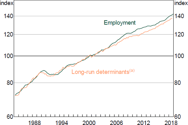
In the long run, employment is determined by a standard labour demand equation that depends on output, the real wage and labour productivity (Figure 11).[23] The equation is similar to those described in Debelle and Vickery (1998) and Hutchings and Kouparitsas (2012). Along a balanced growth path, the wage share is stable and employment grows at the rate of output growth less growth in labour productivity and average hours. This relationship implies a long-run coefficient of one on output, and negative one on trend productivity and average hours. The coefficient on the wage share represents the elasticity of substitution between labour and capital, which indicates how much employment will respond to changes in real wages that cannot be explained by productivity.
In the short run, employment growth has an inertial component and also depends on the recent growth rates of labour costs and GDP. We address concerns of endogeneity in the contemporaneous output and real wages growth terms by estimating the equation using instrumental variables, using lags of the growth of the unemployment rate and labour costs as instruments.
Note: (a) Includes wage share and trend growth variables
Sources: ABS; Authors' calculations
4.8.2 Unemployment rate
We model the unemployment rate using the Okun's Law approach described in Lancaster and Tulip (2015). This relates changes in the unemployment rate to changes in GDP growth relative to a time-varying trend. The change in the unemployment rate also contains an inertial component and depends additionally on growth in real unit labour costs. The latter variable captures the tendency for firms to substitute away from labour when that factor of production becomes more expensive.
As in Lancaster and Tulip, we use a state-space model to estimate time-varying coefficients on lags of changes in the unemployment rate and trend GDP growth. In estimation, we assume that both of these trends follow a random walk.
We project changes in the unemployment rate using the estimated measurement equation from the state-space model. In projections, we hold constant at its last estimated value. The measure of trend growth in the unemployment equation, tyt, is the growth rate that keeps the unemployment rate constant. This rate can differ from the definition of potential GDP growth described in Section 4.1. In forecasts and projections, we converge tyt from its final value towards the standard definition in the model, which is the sum of growth in labour productivity, population and average hours.
4.9 Interest and Exchange Rates
4.9.1 Monetary policy reaction function
In light of the well-known difficulties in estimating the parameters of monetary policy reaction functions (Mavroeidis 2010), MARTIN's baseline specification features a calibrated reaction function in which the overnight cash rate responds to year-ended inflation, the unemployment gap and the change in the unemployment rate:
The variable RSTARt is the time-varying neutral interest rate, which is constructed using the approach described in McCririck and Rees (2017). This variable accounts for much of the decline in the real cash rate over recent decades.
We use the unemployment gap as a measure of spare capacity rather than the output gap for three reasons. First, the unemployment gap is conceptually closer to the RBA's mandated objective of full employment than the output gap. Second, in practice most of the variation in Australian output gap measures comes from variation in the unemployment gap. Third, the unemployment gap is arguably better measured than the output gap. We choose the parameters of the reaction function to provide a reasonable description of the change in the cash rate during several key economic episodes over the past 25 years, including the 1994–95 tightening cycle, the Asian financial crisis and the global financial crisis.
4.9.2 Other interest rates
Changes in the cash rate influence economic activity and inflation largely through their effect on other interest rates in the economy. The most important interest rates in MARTIN are mortgage rates, business lending rates and two-year government bond yields.
The mortgage interest rate is equal to the cash rate plus an interest rate spread. The spread follows an AR(1) process. We include a break in the mean of this spread in early 2008, to capture the increase in mortgage interest rates that occurred following the global financial crisis.
The business lending rate is equal to the cash rate plus an interest rate spread. The spread follows an AR(1) process and also depends on the level of the unemployment gap. The latter variable accounts for the fact that business lending spreads tend to be countercyclical.
Two-year government bond yields depend on the current level of the cash rate and expectations of its future level (proxied by the neutral real interest rate plus inflation expectations):
Real interest rate measures appear in many of MARTIN's equations. We calculate these measures by adjusting nominal interest rates for year-ended trimmed mean inflation.
4.9.3 Real trade-weighted index
We model the real trade-weighted index (TWI) exchange rate using an ECM framework as in Hambur et al (2015). In the long run, there is a cointegrating relationship between the real TWI, the terms of trade and the spread between Australian and G3 real two-year government bond rates. In the short run, changes in the terms of trade and the government bond spread also influence the real exchange rate.
4.10 Foreign Sector
MARTIN's foreign sector is parsimonious and is made up of a small number of exogenous variables, including major trading partner (MTP) GDP growth, various world prices and the interest rates of major advanced economies. These foreign variables affect domestic variables such as exports, imports and the real TWI.
In the long run, we assume that the growth rate of real MTP GDP converges to Australia's trend GDP growth rate. Similarly, growth in foreign prices converges to the Australian inflation target. Foreign policy rates converge to an exogenous estimate of the foreign neutral interest rate, while longer-term interest rates converge to the policy rate plus an estimated term premium.
The foreign block is another area where a tension arises between matching the data and ensuring desirable model properties. For example, the restriction on foreign economic growth is strongly at odds with recent history – on a trade-weighted basis, the GDP growth rates of Australia's major trading partners have exceeded Australian GDP growth over recent decades. However, for a stable balanced growth path to exist either the growth rate of foreign GDP must converge to the growth rate of domestic GDP or relative prices between Australian and foreign goods must drift at a rate that exactly offsets the growth differential.[24] Imposing a slow convergence of foreign GDP growth to Australian GDP growth turned out to be a simpler approach, with fewer implications for the model's dynamic properties, than imposing arbitrary restrictions on the drift of relative prices and the size of trade price elasticities.
While including a more sophisticated foreign sector in MARTIN would have some advantages, we favoured a simpler approach because MARTIN is intended to be a model of the Australian economy. When and if we need more detail on foreign variables, we can supplement MARTIN with other models that have more developed foreign sectors.[25]
Footnotes
In some cases, shorter estimation samples also reflect data limitations. For example, data for the wage price index is available only from 1997. The online appendix lists the estimation sample used for each variable. [11]
We use labour productivity, which accounts for both ‘pure’ productivity growth and capital deepening, because it is subject to less measurement error at a quarterly frequency than alternative concepts such as multifactor productivity. For long-run scenarios and forecasting this choice makes little difference. However, it does limit MARTIN's ability to analyse the short-run effects of changes in productivity growth. [12]
To the extent that asset markets are forward looking, net wealth accounts for the effect of anticipated future income growth on consumption. There is some evidence of the permanent income hypothesis holding empirically in Australia using microeconomic data (e.g. Berger-Thomson, Chung and McKibbin 2009; Kaplan, La Cava and Stone 2018). [13]
Including factors that may influence the risky asset share – such as risk aversion, equity risk premia and equity price volatility – is left for future work. [14]
This implies that other components of the cost of owning are stable and captured by a constant in the long-run levels equation. This is broadly consistent with the evidence presented in Figure 1 of Fox and Tulip (2014). [15]
The remaining components of the cost of capital consist of the weighted average of the cost of debt and equity financing, adjusted for depreciation and the taxation of corporate profits less allowances for depreciation. [16]
In most theoretical models, the coefficient on the user cost of capital in an investment equation is equivalent to the elasticity of substitution between capital and labour, and hence is equal to the coefficient on real wages in a labour demand equation. [17]
Appendix A contains the details of this estimation. An alternative way to deal with drifting export shares would be to include time trends in the exports equations. We prefer to use time-varying constants because the types of structural change we are seeking to capture are unlikely to have had a stable effect on exports growth over time and so are better modelled using a more flexible specification. [18]
The import-adjusted demand measure is based on import penetration ratios calculated from the ABS input-output tables (see Lovicu (2017) for more details). [19]
This variable is the imported consumption good implicit price deflator. [20]
In particular, large increases or decreases in prices (which will tend to be excluded from trimmed mean inflation) will still be relevant for the long-run relationship between the price level and input costs. [21]
The tendency for productivity growth to be faster in the traded sector than the non-traded sector is known as the Balassa-Samuelson effect. [22]
This relationship can be derived by solving the profit maximisation of a firm facing a constant elasticity of substitution production function that takes wages and prices as given. [23]
If this were not the case, then the faster average growth rate abroad would mean that export volumes would increase faster than domestic GDP, which would be inconsistent with balanced growth. [24]
For example, Guttmann et al (2019) uses MARTIN in conjunction with the Oxford Economics Global Economic Model to examine spillovers from the Chinese economy to Australia. [25]