RDP 2019-05: Cost-benefit Analysis of Leaning against the Wind 5. Extensions
July 2019
- Download the Paper 1,513KB
Results like those in Figure 3 are common and appear in various forms in different papers. However, they rest on some simplifying assumptions. In this section we discuss some complications. These generalise and make more realistic the earlier results without changing their essential character. Several of these extensions address criticisms of the simple approach. These criticisms can be quantified and they turn out not to change the conclusions.
5.1 Leaning against the Wind is More Desirable When Risks Are High
Many proponents of leaning against the wind call for it to be applied in response to rapid growth in credit or asset prices (e.g. Borio and Lowe 2002). As the name of the policy implies, it is selectively applied when risks are expected to be high. It is implicitly assumed that the benefit-cost ratio rises above 1 as financial risks increase.
The results in Sections 2 and 3 do not clearly assess such a policy, because the dependence of the estimates on financial conditions was not explicit. On a simple reading, many of the cost-benefit comparisons may appear to test whether leaning against the wind is either always desirable or never desirable. In this section we make underlying parameters conditional on financial conditions, to address the question ‘When is leaning against the wind desirable?’ Or, more bluntly, ‘Which wind?’
To be clear, the relevant question is not whether the probability of a crisis varies (though it does). To justify variations in policy over time, the response of costs or benefits to interest rates needs to vary. We focus on variations in the effect of interest rates on the probability of a crisis. Because interest rates operate through credit growth, this means the central question is whether the effect of credit on the probability of a crisis varies with financial conditions.
5.1.1 When real credit growth is high
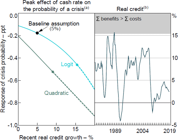
Schularick and Taylor's (2012) preferred specification is a logit model. This is nonlinear, with interest rates having a larger effect on the probability of a crisis if real credit is growing at a faster pace. The aqua line in Figure 5 (left panel), labelled ‘Logit’, shows the marginal effect of the cash rate on the probability of a crisis, which becomes more negative as real credit growth increases.
The analysis underpinning Figure 3 estimated that a higher cash rate reduces the probability of being in a crisis by 0.2 percentage points at its peak, assuming that real credit growth was 5 per cent per annum over the previous five years. This is shown as the black dot, labelled ‘Baseline assumption’ in Figure 5 (left panel). Sensitivity analysis suggests that the benefits of leaning against the wind would exceed the costs if the effect on the probability of being in a crisis was doubled, peaking at –0.4 percentage points. This threshold is reached when real credit grows by around 15 per cent per year, shown as the aqua dot. As shown in the right panel of Figure 5, real credit has usually grown much slower than this threshold, though it briefly exceeded it in the late 1980s.

Notes:
(a) Estimates include Australia-specific intercepts (i.e. fixed effects); dashed lines represent rates of
real credit growth for which the benefits of leaning against the wind exceed costs
(b) Year-ended growth
Sources: ABS; Authors' calculations; Schularick and Taylor (2012)
The nonlinearity in our estimates could reasonably be argued to be a result that is assumed rather than estimated, and that it is an accidental by-product of a functional form chosen for other reasons. However, a specification chosen so as to directly model the argument for nonlinear effects gives similar results. We estimate a least squares version of Schularick and Taylor's model, in which the probability of a crisis is a linear function of five lags of squared real credit growth.[11] These terms are jointly significant with a p-value of 6 per cent. That is, the statistical significance of these nonlinearities is marginal. The partial derivative of the probability of a crisis with respect to interest rates, shown as the dark aqua line in the left panel of Figure 5 (labelled ‘Quadratic’) then linearly decreases with credit growth. Although the quadratic specification is less plausible than the logistic, it has similar policy implications: leaning against the wind would be justified when credit growth is very high (for the quadratic specification, 9 per cent per year), well above current rates of growth.[12]
5.1.2 When the credit gap is high
A closely related hypothesis is that leaning against the wind is worthwhile when the credit-to-GDP ratio is high. This is one interpretation of the argument of the BIS (2016) that monetary policy should respond to ‘the financial cycle’. Borio (2016, p 5) argues that policy responses to the ‘cycle’ also apply to the credit gap, which is a major element of the BIS's cycle indicator. The credit gap is also a widely used early warning indicator of financial crises, and is required under the Basel III rules to be reported in the course of setting the countercyclical capital buffer (APRA 2015).
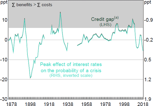
To assess whether leaning against the wind is more desirable when credit is high, we replace the squared terms in the least squares probability model of the previous section with both the level of the detrended credit-to-GDP ratio, or credit gap, and the product of the credit gap and real credit growth, both lagged two years. This interaction term allows the effect of real credit growth on the probability of a crisis – and hence the benefits of leaning against the wind – to increase linearly with the credit gap. The interaction term has a p-value of 4 per cent.[13] This effect is quantified in Figure 6, which shows the level of the credit gap on the left axis. The peak effect of the cash rate on the probability of a crisis is shown on the right axis. This is the same variable as shown in the left panel of Figure 5, however, as the effect is linear, we simply show this by rescaling the axis. Substituting this specification into the analysis underlying Figure 3, leaning against the wind would be worthwhile if the peak effect of the cash rate on the probability of a crisis was larger in magnitude than –0.6, which would occur if the credit-to-GDP ratio was 6 percentage points above trend, a level it last reached in 2003. We return to this issue in Section 6.3.

Note: (a) Deviation of credit-to-GDP ratio from one-sided HP trend with smoothing parameter of 1,562.5.; this is equivalent to the smoothing parameter of 400,000 recommended by the Basel Committee on Banking Supervision (BCBS) for quarterly data (Ravn and Uhlig 2002)
Sources: ABS; Authors' calculations; Schularick and Taylor (2012)
Higher interest rates reduce the probability of a crisis by lowering credit growth, which is estimated to have a larger effect on the probability of a crisis when the credit gap is higher. In principle, the credit gap could have further effects on the probability or severity of a crisis. We discuss these effects in Section 6.2.
5.2 Severity of the Crisis Depends on Policy
Sections 2 and 3 assumed that a crisis results in an unemployment gap of 5 percentage points, which was independent of other factors. However, as we discuss in this section, the severity of a crisis may be affected by a policy of leaning against the wind.
Svensson (2017a) suggests that a crisis is more likely to result in a fixed increase in the unemployment gap than a fixed level. Results shown in Figure 2 appear to be consistent with this. Starting from a higher pre-crisis unemployment gap, a crisis of a given size would result in a higher peak unemployment gap. Assuming increasing marginal costs (for example, quadratic loss), this increases the welfare cost of leaning against the wind. That is, the cost of leaning against the wind is not just a weaker economy if no crisis occurs, but a more costly crisis if it does occur.
Table 2 shows benefit-cost ratios based on some alternative assumptions that have been used in the literature. The first row represents our earlier estimates shown in Figure 3. The next row allows the severity of a crisis to depend on the pre-crisis unemployment gap. In Appendix B we explain how this effect, and others discussed below, can be estimated. Assuming that a crisis increases the unemployment gap by 5 percentage points (instead of to 5 percentage points) lowers the benefit-cost ratio to 0.07.
| Assumption | Benefit-cost ratio(a) | |
|---|---|---|
| 1 | Baseline: unemployment gap is 5 percentage points | 0.31 |
| 2 | Unemployment gap increases by 5 percentage points from the gap just before the crisis | 0.07 |
| 3 | Unemployment gap depends on recent credit growth | 0.62 |
| 4 | Unemployment gap depends on both pre-crisis unemployment gap and recent credit growth | 0.14 |
|
Notes: Appendix A shows how the total loss is decomposed into
separate benefits and costs for each of these assumptions; |
||
In contrast, Gerdrup et al (2016) find that a crisis is likely to be more severe if real credit was growing strongly before the crisis. So by lowering credit growth, leaning against the wind is likely to decrease the severity, as well as the probability, of a crisis. For illustrative purposes, we use Gerdrup et al's estimates to gauge the relationship between credit growth and the severity of a crisis, shown in row 3 of Table 2. This increases the benefit-cost ratio to 0.62.
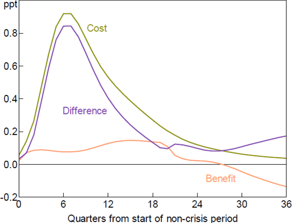
Row 4 and Figure 7 combine both assumptions. The severity of a crisis is much more affected by a higher initial unemployment gap than by slower growth of real credit. Allowing for both effects results in a benefit-cost ratio of 0.14; costs are eight times benefits. This is our preferred estimate.[14]

Footnotes
A possible issue with including squared real credit growth is that it does not distinguish between falls and increases in real credit. To address this issue, we have set the squared terms equal to zero when real credit growth is negative. [11]
The different levels of the lines in the left panel of Figure 5 are due to the low Australia-specific intercept, which depresses the marginal effect of interest rates in the logit equation but not in the linear probability model. Estimates from a logit model without country-specific intercepts are similar to the quadratic specification, with benefits equalling costs when real credit grows at 8 per cent. [12]
To avoid constraining the functional form, we also include the lagged credit gap as a separate regressor, which has a p-value of 46 per cent. Similar to the regression with squared credit growth, we restrict the interaction term to be zero when both the credit gap and real credit growth are negative. This restriction is not important; we get similar results if we use either the unrestricted interaction term in the regression, or if we add an arbitrary constant to the credit gap so that it is always positive. [13]
Figure 7 shows a negative ‘benefit’ after a period of seven years (the light orange line). This reflects the response of real credit to the assumed path for interest rates, which turns positive once interest rates are below their baseline level. The higher level of real credit growth increases the expected severity of a crisis, which is included as a negative benefit. [14]