RDP 2019-05: Cost-benefit Analysis of Leaning against the Wind 3. Dynamic Estimates for Australia

A limitation of the simple approach used in Table 1 is that it ignores the evolution of costs and benefits over time. Because the elements interact multiplicatively and the loss function is quadratic the problem is highly nonlinear, so simple averages can be misleading. In this section, we show dynamic estimates for Australia which address this issue. We draw on the relevant research for each step in the argument, which comes from different sources and uses different methods. Joint estimation would be possible (Pescatori and Laséen (2016) is an example), however, we judged it to be more transparent and credible to use models and results that, where possible, have already been published and scrutinised. We also compare our estimates with others in the international literature. In general, the estimates seem to be similar, with differences being small and offsetting.

We show estimates over a nine-year horizon, the window most favourable to leaning against the wind. Assuming that monetary policy does not affect real variables in the long run, real credit growth would be above baseline (to get back to equilibrium) if the horizon were lengthened. That would reverse many of the effects shown below, driving the sum of total effects towards zero.

3.1 Interest Rate Assumption

To find a plausible profile for leaning against the wind, we take the difference between a forecast of the Australian economy in which interest rates evolve in line with market quotes and an optimal control scenario. The forecast based on market quotes closely resembles the forecast in the May 2016 Statement on Monetary Policy (RBA 2016b). The optimal control scenario sets interest rates so as to minimise the squared deviations of inflation from its target, the unemployment rate from the NAIRU, and squared changes in the policy rate. This optimal control exercise is much the same as those discussed in Stone, Wheatley and Wilkinson (2005, Section 3.3), Yellen (2012) and Haldane (2015). The key difference between the scenarios is that the forecast using market interest rates allows monetary policy to lean against the wind, whereas optimal control does not. Both scenarios are generated by the AUS-M model maintained by Outlook Economics.^[3] The IMF (Habermeier et al 2017, p 46) provide and discuss similar estimates.

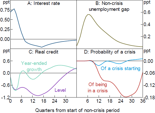
As shown in Figure 1A, this approach results in the cash rate being around 70 basis points higher for a period of a year, after which it declines to be around 25 basis points lower. We take this path of interest rates as given and examine the effects of leaning against the wind by this magnitude.

3.2 Response of the Non-crisis Unemployment Rate

The non-crisis unemployment gap is expected to increase by slightly more than ½ percentage point over a two-year period in response to the higher cash rate, before it gradually returns to its baseline level (Figure 1B). This estimate represents the difference between the unemployment rate projections in the ‘market path’ and ‘optimal control’ scenarios discussed above. AUS-M's estimate of the effect of interest rates on the rate of unemployment is slightly stronger than estimates for some other countries.^[4] It is not clear whether this reflects differences between models or differences between countries. As with most macroeconometric models, AUS-M does not have a detailed financial sector, and so does not provide estimates of many of the other relationships in which we are interested. However, models of its type are a standard method of estimating the effect of interest rates on unemployment. For our purposes, they have the added advantage of providing consistent optimal control estimates.

Leaning against the wind affects many other variables that society cares about, such as inflation, income, the budget deficit and so on. Several papers use more comprehensive measures of costs. For example, Ajello et al (2016) and Pescatori and Laséen (2016) use a quadratic loss function that includes both the unemployment rate and inflation rate. However, if other variables move in line with unemployment, then both benefits and costs would increase proportionately and the ratio would be unchanged. The main challenge to this assumption is that crises may have permanent effects on output, which we discuss in Section 6.1.

3.3 Response of Real Credit

The baseline structural VAR described in Jacobs and Rayner (2012, pp 19–21) may provide the most authoritative estimates of the effect of real interest rates on credit in Australia.^[5] This VAR implies that the 75 basis point increase in interest rates shown above would reduce the pace of growth of real credit by 0.9 percentage points after one year (Figure 1C). The pace of the decline slows as higher interest rates are unwound, and becomes positive once interest rates are below their baseline level. The level of real credit returns to its baseline level around eight years after the initial increase in interest rates. This response of credit is similar to or slightly larger than various international estimates. It is near the average of seven estimates surveyed by Gerdrup et al (2017, Table 1), that is, a 1 per cent increase in interest rates reduces credit by 1.35 per cent. Our estimated response is slightly larger than the estimates used by Svensson (2017a, Figure 3), and is near the upper end of a range of estimates in the international literature surveyed by the IMF (Habermeier et al 2015, fn 19). It is much larger than the ‘TOTEM’ and ‘Lens’ estimates reported by Gorea et al (2016, Figure 2) but somewhat smaller than their ‘MP2’ estimates.

We also experimented with other VARs used for operational work within the RBA. These are simpler than the model of Jacobs and Rayner (2012) and estimate a smaller effect of interest rates on credit. Results are available in the online supplementary information accompanying this paper. In order to show leaning against the wind in a more favourable light, we use the VAR that shows the larger effect.

The literature on leaning against the wind assumes that it is the growth in real credit that affects the probability of a banking crisis. Research underpinning that assumption is discussed in the following section. Alternatives to that assumption are discussed in Section 6.2.

3.4 Response of the Probability of a Crisis

The preferred model of Schularick and Taylor (2012) predicts the probability of a financial crisis starting as a function of five lags of annual real credit growth. According to this model, the probability of a crisis occurring in Australia has recently ranged from a peak of around 12 per cent in 1991 to 6 per cent in 2007 (prior to the GFC) and to a low in 2015 of about 3 per cent.^[6] These estimates, particularly those for Australia before the crisis of the early 1990s and before the GFC for other countries, strike some as surprisingly low. That partly reflects a view that these crises were predicted beforehand by some observers. It may also reflect ‘hindsight bias’, the well-documented tendency to think that past events were more predictable than they actually were. See Wikipedia (2006) and references cited therein.

Schularick and Taylor's estimates seem to be fairly robust. Qualitatively similar results are obtained by the IMF (Habermeier et al 2015, p 17) for 35 advanced countries from 1960, by Babecký et al (2012) for 40 developed economies from 1970, by Gerdrup et al (2017) for 20 OECD countries since 1975, by Aikman et al (2018) for 23 developed countries since the 1980s, and by Kockerols and Kok (2019) for 22 European countries since 1970. There are considerable differences in specification and data measurement across these papers. They and others, such as Pescatori and Laséen (2016) or Svensson (2017a), conduct substantial sensitivity analysis.

For the purposes of assessing policy, it is the change in probability arising from new conditions, not the level, that matters. Schularick and Taylor's model, together with the lower credit growth discussed in the previous section, would imply that the quarterly probability of financial crises starting troughs at 0.02 percentage points below the baseline, as shown by the light blue line in Figure 1D.^[7]

The ability of these models to predict financial crises, let alone changes in their probability, is very weak. But this does not mean the models are uninformative. We can confidently reject the hypothesis that the effects of changes in credit are large. If these effects were large, the models would have more explanatory power. A corollary of crises being unpredictable is that it is difficult to prevent them, although fostering resilience might be feasible.

The probability of being in a crisis (the red line in Figure 1D) represents the probabilities of a crisis starting in a given quarter, summed over the assumed duration of a crisis.^[8] This troughs at 0.18 percentage points below the baseline. This is slightly larger (in magnitude) than the middle of the range of estimates reported by the IMF (Habermeier et al 2015, p 18), which range from −0.04 to −0.3 percentage points in response to a 1 percentage point interest rate increase.^[9]

To put this in context, financial crises, as defined by Schularick and Taylor (2012), have occurred twice in Australia since 1870 – starting in 1893 and 1989. If we assume these crises lasted for six years, the unconditional probability of being in a crisis at any given point in time is 8.3 per cent. A reduction of 0.18 percentage points would lower that probability to 8.12 per cent. The tiny size of that change deserves emphasis. It implies that leaning against the wind is fairly ineffective at reducing the risks of financial crises. Its benefits are small – both relative to the costs of the policy (quantified below) and relative to the effects of other policies that might be employed (see, for example, Firestone, Lorenc and Ranish (2017)).

The small estimated effect of interest rates on the probability of financial crises has surprised many people. However, it is implied by central features of the data. Interest rates and credit growth vary over a wide range over the typical business cycle. So if interest rates or credit growth had substantial effects on the probability of a crisis then we would have experienced repeated episodes with a significant probability of a crisis. However, financial crises have been rare. In Australia they have been once-in-a-lifetime events.

3.5 Unemployment Gap in a Crisis

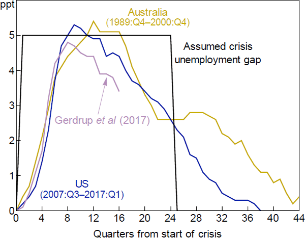
Figure 2 shows estimates of the change in unemployment during a financial crisis. The yellow line represents Australia from 1989^[10], the blue line shows the United States from 2007 and the violet line shows average estimates by Gerdrup et al (2017, Figure 1) for a panel of 20 OECD countries from 1975 to 2014. We assume that in the event of a crisis the unemployment gap is 5 percentage points for six years, the same assumption the IMF made in Table 1 above. The IMF suggests this is representative of previous crises. This assumption, shown as the black line in Figure 2, describes a somewhat more severe crisis than the other estimates shown. Again, we choose parameters that favour leaning against the wind.

3.6 Comparing Costs with Benefits

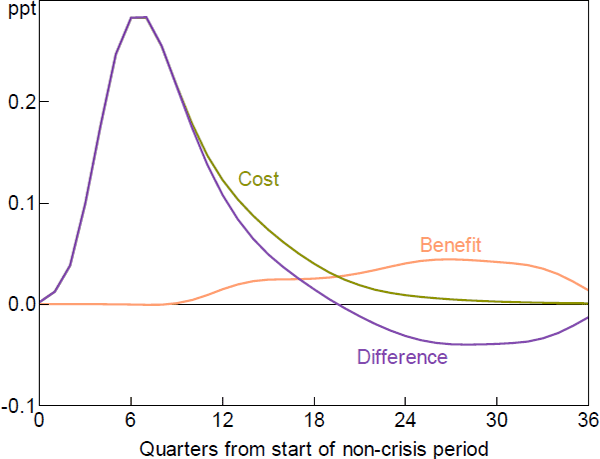
Figure 3 puts the above elements together. Expected loss is a probability-weighted average of the crisis and non-crisis losses. Appendix A shows how this loss can be decomposed into separate costs and benefits. The expected costs of leaning against the wind are given by Equation (A4) and represent the higher unemployment directly arising from higher interest rates (shown in Figure 1B), squared, with a small adjustment reflecting relative probabilities. Expected benefits are calculated using Equation (A5) and represent the increase in the squared unemployment gap in a crisis (that is, the difference between the assumed crisis unemployment gap – 5 percentage points – and the line in Figure 1B) multiplied by its lower probability (the red line in Figure 1D).

Figure 3 shows the flow of costs and benefits. We then sum these over a nine-year horizon, given most costs and benefits have accrued within this time frame. For simplicity, we assume the discount rate is zero. Our results are not very sensitive to alternative discount rates.

Both benefits and costs are in essentially the same units as in Table 1, so it is easy to compare Figure 3 with the IMF survey and the research on which it draws. The main difference between the dynamic and static estimates is that the response of the probability of a crisis, shown as the red line in Figure 1D, changes noticeably over time. In contrast, the estimate of the change in this probability in Table 1 is the peak effect of a range of estimates, which will overstate the benefits of leaning against the wind. This illustrates the benefit of a dynamic approach.

Nonetheless, the central result is the same as in the simple analysis of Table 1: costs greatly outweigh benefits. In the nine years following the initial increase in interest rates, the costs of leaning against the wind are estimated to be over three times larger than the benefits.

Footnotes

Both scenarios use data as of April 2016. The AUS-M model is not publicly documented, however, its macroeconomic properties are essentially the same as those of the earlier TRYM model, discussed in detail at <http://archive.treasury.gov.au/contentitem.asp?NavId=016&ContentID=238>.

The RBA has developed a new macroeconometric model, MARTIN (see Cusbert and Kendall (2018)). Most of the work for this paper was done before MARTIN became operational.

[3]

In response to a 100 basis point increase in the policy rate for a year, the IMF's GIMF model implies a peak increase in unemployment of somewhat less than ½ percentage point. The IMF (Habermeier et al 2015) describes this as broadly consistent with estimates from other models. The IMF's scenarios (for example, that shown in Table 1) assume this peak effect is constant for four years, implying a more persistent response than AUS-M. The Riksbank's DSGE model, Ramses, suggests that following a 100 basis point increase in the policy interest rate that is maintained for a year, Sweden's unemployment rate would also increase by about ½ percentage point after six quarters, before slowly falling back towards its baseline level (Svensson 2017a, Figure 1). These responses are somewhat weaker than that shown in Figure 1B given that the latter is in response to a 75 basis point interest rate change. [4]

This VAR includes gross national expenditure, GDP, inflation, the cash rate, interest rate differentials, real business credit, a survey measure of difficulty obtaining finance and the real exchange rate as endogenous variables, and major trading partner GDP, real commodity prices and real foreign interest rates as exogenous variables. The contemporaneous matrix is non-recursive. [5]

More detailed results are in our online supplementary information. Thanks to Matt Read for these calculations. [6]

This estimate uses the Australia-specific intercept, using Schularick and Taylor's online database and code (available at <http://economics.ucdavis.edu/people/amtaylor/files/CreditBoomsAER_data_replication.zip>), and assumes that real credit grows at 5 per cent a year in the absence of leaning against the wind, approximately the growth rate when we did this analysis (Figure 5, right panel). We discuss estimates conditional on other variables in Section 5.1. [7]

As discussed by Svensson (2017a, Appendix C), this is a linear approximation of the probability of a crisis, which is simple to calculate but results in slightly larger estimates of the crisis probability. A more thorough approach would be to model the probability of a crisis as a Markov process. [8]

Schularick and Taylor (2012), on which our results are based, describe a one standard deviation (7 percentage points) increase in real credit growth as increasing the incidence of financial crises by 2.8 percentage points. The estimates in Figure 1D are smaller because they reflect a much smaller change in credit growth (Figure 1C). [9]

Movements in the Australian unemployment rate to 1996 are perhaps more representative. After that, interest rates started to increase, signalling the beginning of a new business cycle. [10]