RDP 2019-02: Is Declining Union Membership Contributing to Low Wages Growth? 4. Is There a ‘Union Wage Growth Premium’ and Has This Shrunk over Time?
April 2019
That the share of the workforce covered by enterprise agreements negotiated with union involvement has not changed materially over time suggests that the declining union membership rate has played only a limited role in the recent slowing in wages growth. Lower membership rates may nevertheless put downward pressure on wages growth insofar as it reduces the ability of unions to extract more favourable wage outcomes from firms. For example, fewer paying members may lead to fewer resources allocated to wage negotiations at the firm level. As such, this section of our paper examines whether the ability of unions to obtain higher wage outcomes changed over recent years.
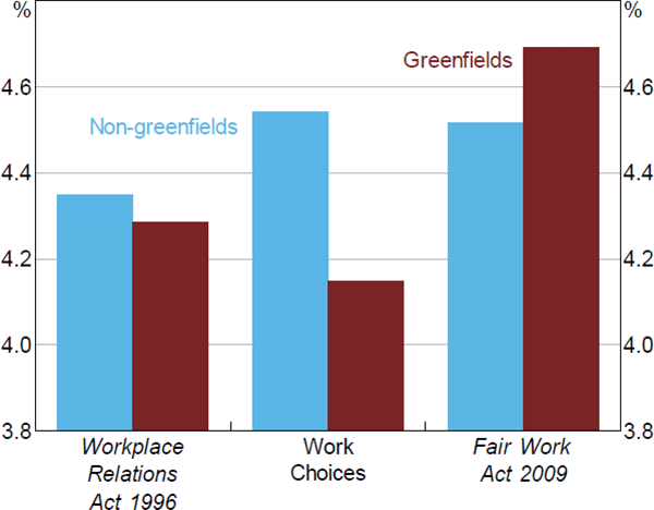
We can examine this question empirically by looking at whether a union wage growth premium exists and, if so, whether this premium has declined over time.[22] Private sector enterprise agreements negotiated with union involvement tend to have higher wage increases than those negotiated without union involvement, while there is little evidence of a similar differential in the public sector (Figure 6).[23] This unconditional difference in wages growth in the private sector appears to have been relatively stable over recent years. Of course, this ‘raw’ difference could be due to inherent differences between union and non-union agreements, rather than a causal effect of union involvement per se. For instance, workplaces that are more profitable on average may also be more likely to have unions involved in their wage negotiations; these workplaces may offer workers larger wage increases even in the absence of union involvement. Our analysis in the following sections attempts to abstract from these inherent differences and, instead, estimate the causal effect of unions on wages growth in collective agreements.
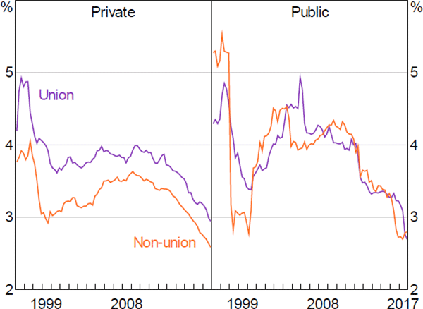
Notes: Agreements in force at quarter-end; weighted by number of employees
Sources: Authors' calculations; Department of Jobs and Small Business Workplace Agreements Database
4.1 Data
To estimate the union wage growth premium we use data from the Workplace Agreements Database (WAD), which is manually compiled by the Department of Jobs and Small Business from administrative data. This rich database includes information on every federally registered enterprise agreement since the early 1990s (subsequently referred to as ‘enterprise agreements’ or ‘agreements’). There are more than 150,000 agreements in the WAD, with around 8,000 new agreements added every year. Data are available on the size and timing of wage increases, the number of employees covered, the industry and state of the firm, and the unions that were involved in wage negotiations (if any).
Given the nature of the WAD, our unit of analysis is the agreement. We also make the case that this is the most appropriate level of analysis for studying union wage effects in Australia. In most cases an agreement will correspond to a single firm, since the vast majority of agreements cover only one employer. But in some cases a single agreement may cover more than one firm (a ‘multi-enterprise agreement’), or there may be multiple agreements covering different groups of workers within a single firm. For the remainder of our paper, we use the terms ‘firm’ and ‘agreement’ interchangeably.
4.1.1 Constructing agreement families
The WAD allows us to follow ‘families’ of agreements over time: that is, sequentially negotiated agreements that cover the same group of workers or positions, usually at a single firm. This means that our data have a panel dimension that enables us to control for any time-invariant characteristics of the firm, such as workplace culture. Our process for constructing agreement families in the WAD can be described using the stylised example in Figure 7.[24]
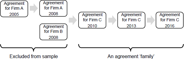
Our first step is to identify the most recent agreement in any given family of agreements (e.g. the agreement for a firm in 2016). We then look at the most recent agreement that the 2016 agreement replaced (e.g. the agreement for the same firm in 2013) and check whether it covered exactly the same group of workers. If so, those two agreements are in the same family. We then check if the agreement that the 2013 agreement replaced (e.g. the agreement for the same firm in 2010) also covered exactly the same group of workers. If so, all three of these agreements are in the same family.
At some point we may find that an agreement covered a different group of workers to its predecessors. In the stylised example in Figure 7, the 2010 agreement replaces two different agreements. For example, Firm A might have merged with Firm B in 2010 and a new agreement was created that covered all employees in the combined Firm C. Because the 2010 agreement covered a different group of workers to earlier agreements, we do not include the 2008 agreements – nor any of the agreements they themselves replaced – in our matched sample. Only the 2010, 2013 and 2016 agreements will constitute a ‘family’ and be included in our matched sample.
Our approach means that more recent agreements are systematically more likely to be included in our matched sample. However, we are still capturing around 85 per cent of all agreements that we can possibly capture in our matched panel.
4.1.2 Measuring wage outcomes
Our measure of the wage outcome from negotiations is the average annualised wage increase (AAWI) over the life of the agreement. The AAWI captures any changes in base pay but not allowances or bonuses paid separately to the base wage. We use the following formula to calculate the AAWI of an agreement:
where wt is the percentage wage increase at time t, N is the number of increases over the life of the agreement, and d is the effective duration of the agreement in years.[25] Effective duration is defined as:
where expidate is an agreement's nominal expiry date, lastincr is the date of the final wage increase in the agreement, certdate is the agreement's certification date, commdate is its formal commencement date, and firsincr is the date of the first wage increase in the agreement. This calculation of the effective duration recognises that certification dates often do not align with the first wage rise (certification sometimes happen after the first wage rise), and that contracts often overlap each other so that the first pay rise of a later contract is granted before the last pay rise of the earlier agreement.[26]
The AAWI calculation is similar to that used in Department of Jobs and Small Business (2018), with a small modification to ensure that the measure is appropriate for modelling. Unlike in the measure used by the Department, we do not use the actual termination date for an agreement as its end date if the agreement is terminated before its nominal expiry date. This is because our research question naturally focuses on the negotiation phase for each agreement: we want to include only information that was available to bargaining participants at the time an agreement was signed and not what happened subsequently. In Section 4.4.2, we consider whether our results are robust to using some alternative measures of wages growth that are adjusted for renegotiation delays.
The WAD does not include information on the wage level in each agreement. As such, we cannot directly estimate the union wage level premium commonly seen in the literature. We discuss the implications of this in Section 4.6.
4.1.3 Sample for estimation
Our baseline models are estimated using a sample of around 46,000 agreements, which is only a subset of the 150,000 or so agreements in the WAD. There are two reasons for this. First, some of the agreements in the dataset do not have a measure of AAWI that was quantifiable at the date the agreement was made. For example, we cannot construct an AAWI in cases where wages are indexed or linked to the consumer price index, to Fair Work Commission award decisions, or to the firm's performance.[27]
Second, in many cases we cannot match an agreement to another in the same agreement family.[28] We exclude these agreements as our baseline estimates of the union wage growth premium are necessarily based only on cases where the same group of workers switch from negotiating with union involvement to negotiating without unions (and vice versa). In Section 4.4.5, we examine if this creates a selection bias by comparing our baseline estimates (with fixed effects) to a simpler model (without fixed effects) estimated using the full sample of all agreements with a quantifiable AAWI.
Descriptive statistics on the estimation sample can be found in Tables B1 and B2.
4.2 Empirical Approach
We use the following model to estimate the effects of union involvement in enterprise bargaining on wages growth:
where the dependent variable is the AAWI for firm i in industry j and state s in the quarter the agreement started, t.[29] The variable of interest (Unionijst) is a dummy variable that equals one if a union was involved in bargaining, and zero otherwise. Xijst is a vector of controls that vary by firm, industry, state and time.[30] The fixed effects (θi) control for any permanent differences in wages growth across firms. The model also controls for the effects of the economic cycle and industry- and location-specific shocks by including the three-way interaction between industry, state and time period (θjst). This absorbs the effects of any macro shocks that affect all firms in any given quarter, along with any time-varying shocks to specific industries or states (or industry-state combinations).
The coefficient of interest (ϕ) measures the union wage growth premium (if positive) or penalty (if negative). The inclusion of fixed effects in Equation (1) means that the union premium will only be identified by variation within firms over time. We will only be able to uncover a positive union wage growth premium if, on average, the size of wage increases shrink when an agreement negotiated with union involvement is replaced by one negotiated without union involvement, or vice versa. Our baseline estimates are not weighted by the number of employees covered by each agreement. We discuss some alternative weighting strategies in Section 4.4.1. Since unions in Australia are typically organised along industry lines and engage with multiple firms, we adjust the standard errors for two-way clustering at the firm and two-digit industry levels.
4.2.1 Potential omitted variable bias
For this approach to yield a causal estimate of the union premium, it is crucial that union involvement is ‘as good as randomly assigned’ given our controls. One concern is that, despite our extensive controls, union involvement could still be endogenous. An agreement negotiated without union involvement could be replaced by one negotiated with union involvement (and vice versa) for unobserved reasons that are also correlated with wages growth. The sign of any bias is unclear ex ante. For example, our estimates will be upwardly biased if employees are more likely to start involving a union in negotiations if they believe that they would receive a favourable outcome from doing so. On the other hand, our estimates will be downwardly biased if employees ask a union to step in to help offset the effect of a sudden reduction in their bargaining power in negotiations.
We address this concern by using a different identification strategy – one that relies on an exogenous change in union involvement introduced by a change in legislation – to estimate the premium. As will be discussed in Section 4.7, we find that the estimated premium using the alternative strategy is larger than the analogous estimate based on Equation (1), but has not changed materially over time.
4.2.2 Transition probabilities
It is also important to consider whether the within-firm variation is limited to only a few firms or confined to a specific period. Among agreement families in our estimation sample that negotiated a new agreement in a given year, the share of agreement families that switched from having union involvement to having no union involvement averaged 3.7 per cent per year in the period leading up to the Work Choices legislative regime (Figure 8). This transition probability rose sharply under Work Choices (2006–09), but declined after Work Choices was repealed and replaced by the Fair Work Act 2009. The share of agreements that switched in the other direction (i.e. no union to union) has averaged 4 per cent since the early 1990s, but has been at above average levels under the Fair Work Act 2009.[31]
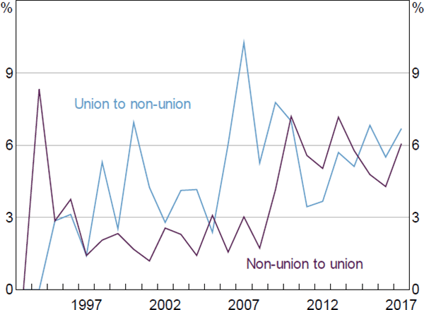
Note: Agreements that have at least one other family member
Sources: Authors' calculations; Department of Jobs and Small Business Workplace Agreements Database
4.3 Baseline Results
Our baseline estimates are shown in Table 1. We present results separately for the private and public sectors. For both sectors, we show results for three specifications, each based on Equation (1): specification (1) does not include the fixed effects or the three-way interaction between industry, state and time; specification (2) omits the fixed effects only; specification (3) is the full model. Comparing the results across the three specifications helps to isolate which controls are important.[32]
With a limited set of controls in the model, union involvement has a strong association with private sector wages growth (Table 1, column 1). This is in line with the persistent unconditional gap in wages growth between union and non-union agreements shown in Figure 6. As column 2 shows, only a small part of the unconditional difference between union and non-union agreements can be accounted for by business cycle factors and idiosyncratic shocks to industries and states. Introducing firm fixed effects – our preferred specification – leads to a further reduction in the size of the union wage growth premium (column 3). The point estimate suggests that annual wages growth in private sector agreements is 0.34 percentage points higher when unions are involved in wage negotiations, relative to when they are not involved. This effect is estimated with a surprisingly small standard error given that we are focusing on variation within firms and within industry–state–time cells. By contrast, we find no evidence of a union wage growth premium in the public sector after accounting for permanent differences between agreement families (Table 1, column 6).[33] Given the absence of evidence for a union wage growth premium in the public sector, the rest of our paper focuses on the private sector union wage growth premium.
| Private sector | Public sector | ||||||
|---|---|---|---|---|---|---|---|
| (1) | (2) | (3) | (1) | (2) | (3) | ||
| Union | 0.64***(0.15) | 0.52***(0.11) | 0.34***(0.09) | −0.03 (0.12) | 0.18** (0.07) | 0.04 (0.04) | |
| Industry–state–time effects? | No | Yes | Yes | No | Yes | Yes | |
| Fixed effects? | No | No | Yes | No | No | Yes | |
| Observations | 41,611 | 41,611 | 41,611 | 4,472 | 4,472 | 4,472 | |
| Adjusted R2 | 0.25 | 0.48 | 0.60 | 0.02 | 0.28 | 0.36 | |
| Adjusted R2 (within) | 0.01 | 0.00 | |||||
|
Notes: ***, **, and * denote statistical significance at the 1, 5, and 10 per cent levels, respectively; standard errors (in parentheses) are clustered at the agreement-family and two-digit industry levels; all specifications control for industry and state Sources: Authors' calculations; Department of Jobs and Small Business Workplace Agreements Database |
|||||||
4.4 Robustness Checks
This section details a number of robustness tests we conduct on our baseline results for private-sector agreements. Readers wishing to continue to the next stage of our analysis may wish to skip to Section 4.5, where we discuss whether the union wage growth premium has changed over time.
The series of robustness tests we conduct, described in Sections 4.4.2–4.4.5 with the results presented in Table 2, often require adding variables that, in many cases, have missing data for some observations. In these cases, we compare the estimates from the robustness model of interest to those from the baseline model estimated over an identical sample. This allows us to abstract from the influence of sample composition between the baseline and robustness samples and isolate the importance of the particular robustness exercise being considered. As such, the ‘baseline model’ estimate in Table 2 differs for each robustness test, but is based on Equation (1) unless otherwise indicated.
| Baseline model | Robust model | Common sample size | Notes | |
|---|---|---|---|---|
| Weighting by employee numbers | ||||
| Union | 0.34*** (0.09) |
0.22*** (0.05) |
41,611 | |
| Accounting for renegotiation delays | ||||
| Union | 0.28*** (0.08) |
0.22*** (0.06) |
19,645 | Sample excludes first agreement in each family |
| Controlling for firm-specific shocks | ||||
| Union | 0.14** (0.09) |
0.15** (0.09) |
7,153 | Sample excludes agreements with missing firm data |
| Controlling for inertia in wage setting | ||||
| Union | 0.23*** (0.07) |
0.18*** (0.05) |
18,795 | Arellano-Bond estimator; includes aggregate time effects only |
| Including unmatched agreements in the sample | ||||
| Union | 0.85*** (0.12) |
94,906 | Excludes agreement family fixed effects | |
| Matched_sample | 0.21*** (0.04) |
|||
| Union × Matched_sample | −0.31*** (0.04) |
|||
| Selection model | ||||
| Union | 0.64*** (0.02) |
0.65*** (0.02) |
45,513 | Heckman model; excludes agreement family fixed effects and time-varying industry and state effects |
|
Notes: ***, **, and * denote statistical significance at the 1, 5, and 10 per cent levels, respectively; standard errors (in parentheses) are clustered at the agreement-family and two-digit industry levels Sources: Authors' calculations; Department of Jobs and Small Business Workplace Agreements Database; Dun & Bradstreet |
||||
4.4.1 Weighting by employee numbers
All agreements are given equal weight in our baseline regressions. An alternative approach is to weight each observation by the number of employees under that agreement. There is little reason to do this on efficiency grounds – our unweighted OLS estimates with robust standard errors are already precise. Rather, weighting may, under some assumptions, get us closer to the population average causal effect of union involvement in the presence of unmodelled heterogeneity of effects (Solon, Haider and Wooldridge 2015). For example, if union involvement tends to have larger effects in the construction industry, then weighted least squares (WLS) estimates that place relatively less weight on smaller agreements – which are more common in construction – will yield a smaller overall premium than OLS. In that case, it may seem that weighting should yield the weighted-average effect of union involvement across the population of employees on enterprise agreements (which is the quantity that we are ultimately interested in for our research question). However, as Solon et al (2015) argue, this is only the case if certain strong assumptions are satisfied; otherwise WLS and OLS are both inconsistent in the presence of unmodelled heterogeneous effects, and neither identifies the population average effect of union involvement.
We find that WLS estimates of the union wage growth premium are smaller than our baseline OLS estimates (0.22 versus 0.34; Table 2). That the differences between OLS and WLS estimates are not large gives us confidence that our baseline results are not being unduly influenced by misspecification bias due to a failure to model heterogeneous treatment effects (Solon et al 2015). We leave the study of heterogeneous effects (e.g. by industry, firm size or union) for future research.
4.4.2 Accounting for renegotiation delays
Our baseline results are based on a measure of wages growth that is similar to the Department of Jobs and Small Business calculation of AAWI. As defined in Section 4.1.2, this measure assumes that the duration of an agreement is the length of time from the start date of the contract to the end date of the contract (the ‘contractual duration’). Any length of time between the end of the firm's previous contract and the start of the current contract (the ‘renegotiation delay’) is ignored. All else being equal, a longer renegotiation delay will reduce wages growth for a group of workers, as wages are often frozen during the negotiation period. Failing to account for these delays could therefore put a bias into our estimates if the length of these delays is related to union involvement in bargaining.
On average, agreements negotiated with union involvement take longer to renegotiate than non-union agreements (Figure 9). After controlling for other factors (using a regression), we find that union involvement in bargaining adds around four weeks to renegotiation delays, compared to when unions are not involved.[34] Since union involvement leads to more protracted wage negotiations on average, our baseline estimates of the union wage growth premium (which do not adjust for these lags) are likely to be biased upwards. However, the size of the bias does not appear to be large: adjusting our measure of AAWI for renegotiation delays yields only a slightly smaller estimate of the union wage growth premium than in the baseline model (0.22 versus 0.28; Table 2).
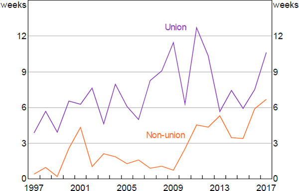
Notes: Weighted by number of employees; excludes agreements that do not replace an existing agreement and those with implied renegotiation delays of more than 18 months
Sources: Authors' calculations; Department of Jobs and Small Business Workplace Agreements Database
4.4.3 Controlling for firm-specific shocks
Our baseline model controls for firm-specific factors that do not vary over time, along with any industry- or state-specific shocks. It does not control for the effects of firm-specific shocks that vary over time. For example, while the model would control for the effects of an industry-wide decline in profits (e.g. due to a decline in industry export prices), it would not control for, say, a profit shock to a specific firm (e.g. due to the retirement of a CEO). If these idiosyncratic firm-level shocks are correlated with changes in union involvement and also with wages growth, we may have omitted variable bias.
We can partially control for firm-level shocks using measures of firm profitability and sales from Dun & Bradstreet. These data are available only for listed companies and can only be linked to the WAD if a firm's Australian Business Number (ABN) is available in both datasets. Unfortunately, ABNs were only routinely recorded in the WAD since 2009, and so we are unable to observe firm-level profit and sales for many firms prior to this.[35] Firm-level data is missing for around three-quarters of all agreements in our sample, which is the reason we did not include these variables in our baseline model. In a model that controls for firm-specific shocks, the union wage growth premium is estimated to be around 0.15 (Table 2). If we re-estimate our baseline model (excluding firm-level controls) using the sample of agreements with non-missing Dun & Bradstreet data, we find a very similar estimate as in the regression with firm-level controls (Table 2). This provides some reassurance that our baseline results are not being driven by idiosyncratic shocks to firms.[36]
4.4.4 Controlling for inertia in wage setting
Our baseline model does not control for the wage outcome in the previous agreement from the same agreement family. Including this variable leads to a large reduction in our sample size: we lose observations both due to the lag itself and because deeper lags of wages growth are needed as instruments. However, excluding this variable may result in biased estimates of the union premium if the firm's previous wage outcome is correlated with workers' decision to negotiate with union involvement. And since wages growth is serially correlated due to inertia in wage setting, omitting lagged AAWI could put a bias into our estimate of the union premium.
To examine the importance of this bias, we re-estimate our baseline model including lagged wages growth as an additional control. We used an Arellano and Bond (1991) estimator to obtain a consistent estimator of the coefficient to lagged AAWI. In this specification the union wage growth premium is only slightly smaller than in the baseline model when estimated over the same sample (0.18 versus 0.23; Table 2).
4.4.5 Sample selection bias
Another potential concern around robustness is that the matched sample of agreements (i.e. those with at least one family member) used in our analysis may not be representative of the broader population of agreements in the WAD. For example, some firms do not have sufficient resources to regularly renegotiate agreements, and as a result are less likely to be included in our matched sample. If such firms also respond differently to union involvement in wage negotiations compared with firms that are matched, then our estimates of the union wage growth premium could be biased. We can examine this issue by estimating a pooled model using the full sample of all agreements – both matched and unmatched – but excluding the agreement-family fixed effects. The estimation sample in this model is more than twice the size of that in the baseline model. We also include a dummy variable that equals one if an agreement is in the matched sample and zero otherwise, and an interaction between this dummy and the dummy for union involvement.
The coefficient of interest is the coefficient on the interaction term, which tells us whether the union premium is different across matched and unmatched samples, conditional on the variables included in the baseline model. We find that this interaction is statistically significant (Table 2). Its sign suggests that the union premium in the unmatched sample is larger than the matched sample. This suggests that our baseline estimates of the union premium may be downwardly biased. However, we show in Section 4.5.1 that these differences between the matched and unmatched samples do not affect our conclusions regarding the role of unions in the decline in aggregate wages growth.
Another sample selection issue is that our baseline model is restricted to agreements whose wage outcomes can be expressed in terms of a ‘quantifiable’ AAWI. This could lead to a selection bias if agreements with a quantifiable AAWI are not a random sample of enterprise agreements (Heckman 1979). For example, workers with less bargaining power may be relatively more willing to agree to wage outcomes that are linked to the consumer price index or to the Fair Work Commission's award decisions (and hence the AAWI cannot be calculated ex ante; see Section 4.1.3 for further details). Union involvement in negotiations may have a different effect for such workers.
We can test for this type of bias using Heckman's two-step procedure to correct for selection bias. In the first stage we model the probability of having a quantifiable AAWI using a probit model. This step requires an ‘excluded instrument’ – that is, a variable that influences whether an agreement has a quantifiable AAWI but does not have a direct effect on the AAWI itself. We use the share of non-expired agreements in the firm's industry that had quantifiable AAWIs in the previous quarter (weighted by firm size) as the instrument. The idea is that a firm's wage-setting practices will be influenced by wage-setting trends in the firm's industry. In the second stage we correct for self-selection by incorporating a transformation of the predicted probabilities from the first stage as an additional explanatory variable in Equation (1).[37] We find no evidence of a selectivity effect (Table 2). This justifies our focus on the sample of agreements with non-missing AAWI in our baseline model.
4.5 Has the Union Wage Growth Premium Changed over Time?
In this section, we use our baseline model to examine whether the influence of unions on wages growth has changed over time. Factors such as the decline in membership rates and changes in the workplace relations system, for instance, may have affected union influence. Any decline in unions' ability to negotiate favourable wage outcomes should manifest itself in a smaller union premium over time.
We can examine the stability of the premium by interacting the Union indicator variable in Equation (1) with dummies for the four major legislative regimes governing the agreements in our sample. These regimes are: the Industrial Relations Act 1988 (1991 to 1996); the Workplace Relations Act 1996 (1996 to 2006); the Work Choices period (2006 to 2009); and the Fair Work Act 2009 (2009 onwards).[38]
The results in Figure 10 suggest there has been little change in the union wage growth premium over time. Indeed, the premium has increased since the Workplace Relations Act 1996 despite the declining union membership rate. We find no evidence of a more recent shift in the union premium: a test for the equality of the coefficients to the interacted indicator variables for Work Choices and the Fair Work Act 2009 cannot be rejected (p-value = 0.704). Indeed, the estimated premium under both of these periods is similar in size to the full-sample estimate.[39] This finding is consistent with studies in the United States and United Kingdom, which also find no evidence of a secular decline in the union wage premium over time (Farber et al 2018; Bryson 2007).
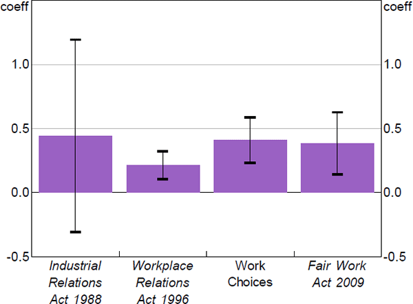
Note: Black lines denote 95 per cent confidence intervals
Sources: Authors' calculations; Department of Jobs and Small Business Workplace Agreements Database
4.5.1 Trends in the unmatched sample
It is important to gauge whether the sample selection issue from our matched and unmatched agreements (discussed in Section 4.4.5) is relevant for estimating changes in the union wage growth premium over time. What ultimately matters for our conclusion that trends in unionisation have not contributed to low wages growth in recent years is whether the difference between the union premiums in the matched and unmatched samples has changed over time. Given our finding in Figure 10 that the union premium has been stable over time for agreements in the matched sample, this boils down to examining whether the premium for the unmatched sample has also been stable.
The union premium for the unmatched sample is more volatile than that for the matched sample (Figure 11). The union premium for the unmatched sample (dark aqua line) has been higher under the Fair Work Act 2009 than under Work Choices. And since the union premium for the matched sample was broadly unchanged across these two legislative regimes (Figure 10; reproduced as the violet line in Figure 11), this implies that a combined sample – pooling both matched and unmatched agreements – would find that the union premium has risen over recent years. This reinforces our conclusion that unionisation has not contributed to low wages growth in recent years.
Note also that the union premium from the unmatched sample (necessarily without fixed effects) is larger than our preferred estimates from the matched sample (with fixed effects). This gap is partly explained by the inclusion of fixed effects for the matched sample: if we omit the fixed effects from our matched sample model, the estimates are closer to the unmatched sample estimates, signalling the presence of unobserved heterogeneity that is positively correlated with wages growth and union involvement (yellow line in Figure 11). However, as discussed in Section 4.4.5 some of the gap is also unexplained.
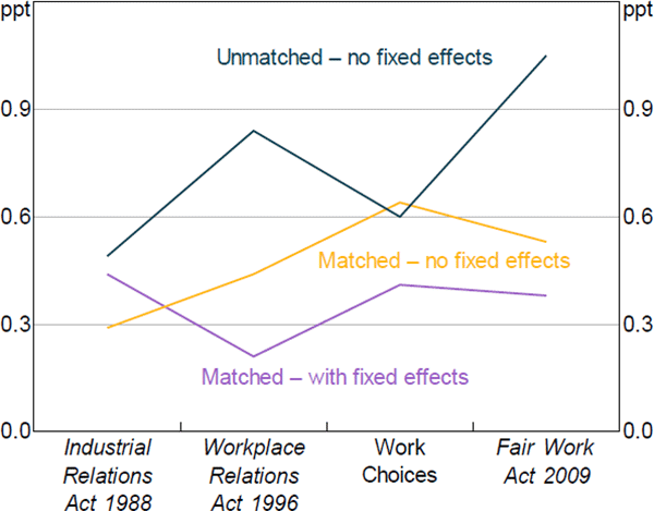
Sources: Authors' calculations; Department of Jobs and Small Business Workplace Agreements Database
4.6 Dynamics of the Union Wage Growth Premium
We have so far discussed the wage growth premium from union involvement in bargaining. However, our baseline results do not reveal how this union wage growth premium evolves over the duration of a union's involvement with a particular agreement family, and what this means for wage levels.
Although our estimates of the union wage growth premium are only identified if an agreement transitions in union status, all wage observations for a given agreement family before and after the transition contribute to the estimation.[40] This means our baseline estimate could be consistent with several possible dynamic paths for wages growth following a change in union status. One possibility is that the union wage growth premium reflects a large one-off spike in wages growth immediately after an agreement changes from no union involvement to union involvement or vice versa, with no further effect on wages growth (relative to the counterfactual of no union involvement) in subsequent negotiations. A stylised example of this case is depicted in the top left panel of Figure 12.
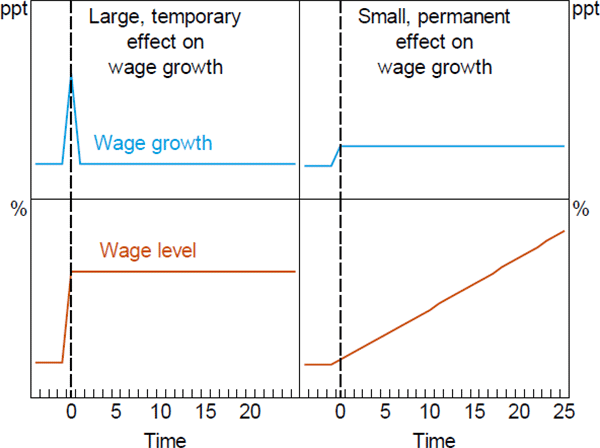
Note: Dashed vertical line denotes year of union entry, t = 0
Another possibility is that our baseline estimates reflect a union wage growth premium (e.g. of ⅓ percentage point per year) that is sustained over all contract negotiations in which a union is involved (top right panel of Figure 12). Although both of these cases can be consistent with our baseline fixed effects estimate of the union wage growth premium, they have different longer-run implications for the level of wages in union, relative to non-union, agreements. These differences are shown in the bottom panels of Figure 12. In the first case (left panels), the adjustment to wage levels from union involvement is immediate, while in the second case (right panels) the adjustment is gradual, with the gap in wage levels between union and non-union agreements widening over time.
We can test which of the two profiles in Figure 12 is most supported by the data by estimating the following equation,
where CUnionijst is a count variable that equals the number of consecutive times an agreement has been renegotiated with union involvement up to time t, after a union first became involved in the negotiations. For instance, this variable would equal one if the agreement becomes the first one in its agreement family to involve a union, and two if the agreement is the second consecutive one in its family to be negotiated with union involvement.[41] If at any point a union is no longer involved in the negotiations, this count variable resets to zero. Given that our baseline union wage premium is identified from both switches from no union involvement to union involvement and switches in the other direction, CUnionijst also counts the number of consecutive times an agreement has been renegotiated without a union after a change in status from union involvement to no union involvement (in this case we multiply the count by minus one).
The immediate effect of union involvement on wages growth – that is, when an agreement negotiated with union involvement replaces one negotiated without a union – is given by ϕ1 + ϕ2. The extent to which this initial wage growth premium then changes over subsequent agreements (conditional on union status remaining the same) depends on ϕ2: a negative estimate for ϕ2 would indicate that the wage growth premium shrinks from the first to subsequent agreements despite ongoing union involvement. In terms of the stylised examples in Figure 12, the left panels would imply a negative value for ϕ2, while the right panels imply ϕ2 is equal to zero.
The results for this specification are presented in Table 3. The coefficient estimates suggest the immediate union wage growth premium is around ⅓ percentage point when union status switches within an agreement family, in line with our baseline results. There is no evidence that this premium changes for subsequent contract renegotiations: our estimate for ϕ2 is close to zero and not statistically significant.[42] That is, ongoing union involvement leads to permanently higher wage growth outcomes. We discuss the implications of this finding below.
| Union | 0.38*** (0.09) |
|---|---|
| CUnion | −0.02 (0.02) |
| Industry–state–time effects? | Yes |
| Fixed effects? | Yes |
| Observations | 41,611 |
| Adjusted R2 | 0.60 |
| Adjusted R2 (within) | 0.01 |
|
Note: See notes to Table 1 Sources: Authors' calculations; Department of Jobs and Small Business Workplace Agreements Database |
|
4.6.1 Implications of the dynamics
The results above suggest that union involvement in bargaining confers a premium in terms of wages growth that is sustained for the duration of the union's involvement with an agreement family. This has implications for the evolution of wage levels. In cases where union involvement does not change over successive agreements, a premium in growth rates implies an increasing premium in levels over time, as wage rises compound (e.g. the lower-right panel of Figure 12). This is the case for most agreements in our sample, as once unions become involved they tend to remain involved. This can be seen in the sample Markov transition probabilities in Table 4.
|
Sources: Authors' calculations; Department of Jobs and Small Business Workplace Agreements Database |
|
Calculating the steady state distribution from these Markov probabilities implies that, in equilibrium, a given agreement family will spend around 96 per cent of the time negotiating with union involvement, and 4 per cent without.
An ever-increasing wage gap between union and non-union agreements is unlikely to be a long-run steady state in the labour market. However, given that our estimate of the union wage growth premium is fairly modest – at ⅓ percentage point per year – a deviation in growth rates could prevail for an extended period of time and still yield a difference in wage levels that is within a reasonable range. Collective bargaining has been a feature of Australia's wage-setting system only since the early 1990s. With this in mind, consider a hypothetical case in which two groups of employees started with the same level of wages in the early 1990s, with only one of those groups receiving a union wage growth premium each year. The difference in wage levels between these groups of workers in 2017 would be around 8 per cent (assuming average wages growth for the group not receiving a union wage growth premium), which is well within the range of estimates of the union premium from studies that focus on wage levels (see Section 2). Our estimates suggest that any current differentials in wage levels between union and non-union agreements reflects the slow accumulation of a modest differential in growth rates over a period of several decades.
Our results are more closely in line with Freeman and Kleiner (1990) and DiNardo and Lee (2004) – both of which consider the short-run effects of new unionisation – than studies using employee-level data, in that our estimates only pertain to recent union entry into negotiations within the past twenty years. Moreover, unlike studies that use a regression discontinuity design, our estimates are identified from a wider population of agreements than those in which the case for union involvement is necessarily only marginal. These reasons help to reconcile our relatively modest estimate of the union wage growth premium with the larger estimates of the union wage level premium from the vast US literature using employee-level data.
4.7 An Alternative Identification Strategy: A Natural Experiment
In this section we use an alternative identification strategy to address concerns about endogeneity in our baseline model. This identification strategy, which exploits a natural experiment that affected union involvement in bargaining for certain types of agreements, should be less susceptible to omitted variables bias (e.g. firm-level shocks that affect both union involvement and wages growth), and as such provides a crosscheck on the fixed effects estimates presented earlier.
4.7.1 The natural experiment
The Work Choices legislation came into effect on 27 March 2006 (amending the Workplace Relations Act 1996), and remained in force until 30 June 2009 when it was replaced by the Fair Work Act 2009. Both the introduction and repeal of Work Choices led to changes in whether a union must be involved in the negotiations of greenfields enterprise agreements. A greenfields agreement is one made in relation to a new business or project, before any workers are employed. Under Work Choices, these agreements could be created without a union – the employer would essentially strike an ‘agreement’ with itself, and a union had no right to demand a seat at the bargaining table (Bray and Stewart 2013). An employer could also choose to make a greenfields agreement with a union. Under the preceding and subsequent legislation, however, greenfields agreements could only be made with a union. These legislative changes are summarised in Table 5, which also shows that there were no changes to rules on whether a union must be involved in non-greenfields agreements during this period.
| Greenfields agreements(a) (‘treatment group’) |
Non-greenfields agreements (‘control group’) |
|
|---|---|---|
| Before Work Choices | Compulsory | Not compulsory |
| During Work Choices | Not compulsory | Not compulsory |
| After Work Choices | Compulsory | Not compulsory |
|
Note: (a) An agreement made in relation to a new business or project, before any workers are engaged |
||
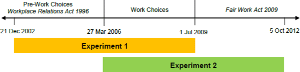
These legislative changes can help us identify the union wage effect in two ways. First, we can study the initial introduction of Work Choices to see if the associated decrease in union involvement in greenfields agreements after March 2006 caused wage growth outcomes in those agreements to be lower (we refer to this as ‘experiment 1’). We can also study the reverse experiment that occurred when Work Choices was repealed in 2009, to see if the associated increase in union involvement in greenfields agreements led to higher wage growth outcomes (‘experiment 2’). In both cases, greenfields agreements are the ‘treatment group’ that is affected by the policy changes governing union involvement in bargaining. The ‘control group’ comprises non-greenfields agreements, which were unaffected by those policy changes on union involvement. For both experiments, we can estimate the causal impact of union involvement on wages growth by comparing the wage outcomes of both groups before and after the policy changes using a difference-in-differences model.
As far as we are aware, beyond the changes to the requirements for union involvement, the legislative changes had no other substantive differential effect on greenfields and non-greenfields agreements.
Prior to Work Choices, our data suggest that all greenfields agreements were made with union involvement, consistent with legislation in place at the time (Figure 13). During the Work Choices period, when union involvement was no longer compulsory for any agreement, the share of greenfields agreements involving a union fell sharply to reach a low of 45 per cent in late 2008. Following the repeal of Work Choices in 2009, union involvement returned to 100 per cent for all greenfields agreements as compulsory union involvement was reinstated for those agreements. By contrast, the rate of union involvement in non-greenfields agreements was little changed over the entire period.
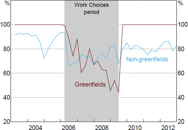
Sources: Authors' calculations; Department of Job lace Agreements Database
4.7.2 Difference-in-differences model
We use a difference-in-differences (DD) approach to study the effect of the two policy changes (in 2006 and 2009) to union involvement on wage outcomes in enterprise agreements. First, to study the effects of the introduction of Work Choices – our ‘experiment 1’ – we estimate the following model:
where the dependent variable is the average annualised wage increase in firm i in period t; the two time periods in t are ‘before’ and ‘after’ the introduction of Work Choices. WCt is a dummy variable that equals one if the agreement was lodged under Work Choices and zero if it was lodged under the previous legislation (the Workplace Relations Act 1996), and Greenfieldsi is a dummy that equals one if the agreement is greenfields and zero otherwise. The coefficient of interest is γ3. Differences in overall average wages growth between greenfields and non-greenfields agreements and changes over time that are common to both groups are captured by γ1 and γ2, respectively. We use data from a symmetric 3¼-year window around the policy change (21 December 2002 to 30 June 2009) for our estimation. [43] Unlike in Equation (1), this difference-in-differences approach does not require a matched sample.
To study the reverse experiment – our ‘experiment 2’ – we estimate the following model, again using a symmetric 3¼-year window around the date of the policy change (27 March 2006 to 5 October 2012):
where the two time periods in t are ‘before’ and ‘after’ the repeal of Work Choices. WCrepealedt is a dummy that equals one if the agreement was lodged after Work Choices was repealed, and zero otherwise. Figure 14 clarifies how the timing of experiments 1 and 2 relates to the relevant legislative changes.
Our earlier finding of a positive union wage growth premium would imply that γ3 is negative and ϕ3 positive. That is, relative to non-greenfields agreements, the annualised wage increases in greenfields agreements should have decreased during Work Choices, and increased with its repeal, because of the associated changes to compulsory union involvement in greenfields agreements. Moreover, assuming that union entry and union exit have symmetric effects on wages growth, our earlier finding that the union wage growth premium has been little changed over time should manifest in estimates of γ3 and ϕ3 that are opposite in sign, but equal in magnitude. We test this below.
4.7.3 Graphical results
Before turning to the results, it is useful to first examine whether there is graphical evidence of an effect of union involvement on wages. Figure 15 compares average wages growth over the three legislative regimes for greenfields and non-greenfields agreements. Agreements with no change to their requirement for union involvement (non-greenfields) saw an increase in wage outcomes during Work Choices, compared to the previous period. In contrast, agreements that shifted from compulsory to voluntary union involvement (greenfields) experienced a decline in wages growth. This is consistent with a positive effect of union involvement on wages growth. Similarly, the gap in wages growth between greenfields and other agreements that emerged during Work Choices was reversed after Work Choices was repealed. Again, this is consistent with a positive union wage growth premium.
Note: Agreements certified between 21 December 2002 and 5 October 2012
Sources: Authors' calculations; Department of Jobs and Small Business Workplace Agreements Database
4.7.4 Difference-in-differences results
The difference-in-differences estimates for Equations (3) and (4) are shown in column 1 of Table 6.[44] Focusing first on the results for experiment 1, the DD estimate suggests that the abolition of compulsory union involvement after 2006 led to a 0.48 percentage point decrease in wages growth in greenfields agreements relative to non-greenfields agreements. As expected, the estimated effect is opposite in sign and only slightly smaller in magnitude (0.44) for the reverse experiment in 2009. A test that the estimates for experiments 1 and 2 are equal in magnitude (but opposite in sign) cannot be rejected (p-value = 0.90).
| Effect of policy change on AAWI (1) |
Effect of policy change on union involvement (2) |
Effect of union involvement on AAWI (3) = (1)/(2) |
|
|---|---|---|---|
| Experiment 1(a) | −0.48*** (0.17) |
−0.23*** (0.07) |
2.14*** (0.63) |
| Experiment 2(b) | 0.44*** (0.16) |
0.28*** (0.07) |
1.59* (0.96) |
| Test of equal effect size (𝑋2)(c) | 0.01 | 4.13 | 0.23 |
| Pr(test statistic > 𝑋2) | 0.90 | 0.04 | 0.63 |
|
Notes: ***, **, and * denote statistical significance at the 1, 5, and 10 per cent levels,
respectively; standard errors (in parentheses) are clustered at the two-digit industry
level Sources: Authors' calculations; Department of Jobs and Small Business Workplace Agreements Database |
|||
4.7.5 Backing out the union wage growth premium
The results in column 1 of Table 6 do not provide a direct estimate of the union wage growth premium. For example, in the case of experiment 1 the DD model yields the average effect of the abolition of compulsory union involvement on wages growth, which would only translate directly into a union effect on wages if the policy change caused the treatment group to go from having compulsory union involvement to having no union involvement at all. This was not the case because although union involvement was not compulsory under Work Choices, many of those agreements did have union involvement (Figure 13). Using experiment 2 as an example, this suggests that in a counterfactual world in which Work Choices had not been repealed, some greenfields agreements would still have been negotiated with a union between 2009 and 2012. That is, some of the agreements that were ‘treated’ after the policy change would still have been treated even if the policy change had not occurred.
To translate our DD estimates into estimates of the union wage growth premium we need to adjust them by an estimate of the share of greenfields agreements whose union involvement was actually affected by the policy changes.[45] We can estimate this share by replacing the dependent variable in Equations (3) and (4) with our dummy variable for union involvement. The results for this specification are shown in column (2) of Table 6. For experiment 1, the point estimates suggest that the abolition of compulsory union involvement due to the introduction of Work Choices induced 23 per cent of agreements to forgo union involvement in bargaining; for experiment 2, the reinstatement of compulsory union involvement (from the repeal of Work Choices) induced 28 per cent of agreements to take up union involvement.
The union wage growth premium can then be obtained by dividing the estimates in column (1) by those in column (2). This estimator is equivalent to an instrumental variable (IV) regression of AAWI on union involvement, where union involvement is instrumented using the DD interaction term.[46] The results, in column (3), imply a union wage growth premium of 2.14 percentage points for experiment 1, and 1.59 percentage points for experiment 2. The difference between these estimates is not statistically significant (p-value = 0.63). This provides us with further evidence that the union wage growth premium has not declined materially in recent years.
The union wage growth premium implied by the DD models is several times larger than the fixed effects estimates in Section 4.3. This could reflect several things. First, it may be that union wage effects are heterogeneous by type of agreement: unions may be able to extract larger wage outcomes from greenfields agreements than non-greenfields agreements. This seems plausible given that, in the absence of union involvement, the baseline level of worker bargaining power across these agreements was very different – under Work Choices an employer could simply strike a greenfields ‘agreement’ with itself, while a non-greenfields agreement still had to be agreed to by its employees. As such, the potential upside in wage outcomes for unions may have been larger for greenfields agreements.[47] The effects could also be heterogeneous among greenfields agreements. This matters because our IV estimator has a local average treatment effect interpretation: it yields the effect of union involvement on wages only for those firms that were induced by the legislative changes to change union involvement status. These firms may have had more bargaining power relative to other greenfields employers, making it possible for them to forgo negotiations with a union and instead set their own terms.
Another possible explanation for the discrepancy between the fixed effects and IV estimates is that one (or both) of these estimators are biased. For example, the fixed effects estimates may be downwardly biased due to omitted, time-varying, firm-level factors that are positively correlated with union involvement but negatively correlated with wages. The DD/IV estimates could be upwardly biased by a macro shock during the Work Choices period that reduced wage outcomes in greenfields relative to non-greenfields agreements (e.g. any shock that differentially affected new businesses, relative to existing businesses). It is nevertheless reassuring that, despite differences in the size of the premium, both identification strategies point to a relatively stable union premium over recent years.
Footnotes
In this paper, any premium associated with union representation would be a ‘pure’ union premium within the subset of employees covered by collective agreements, over and above any (positive or negative) premium associated with collective bargaining. One limitation of our analysis is that we are unable to make more general conclusions about whether the existence and magnitude of this union premium has had wider effects on the likelihood of employers and employees choosing to set pay using enterprise agreements rather than awards or individual arrangements. [22]
The wage growth data reported in Figure 6 – average annualised wage increases – are described in detail in Section 4.1.2. [23]
The WAD provides information on whether an agreement replaces a previous agreement (including its identifier), and whether the group of workers covered by the agreement is the same as the previous agreement. [24]
This method of averaging implicitly assumes that the increases are evenly spaced across the agreement's effective duration. [25]
In the vast majority of cases, an agreement's nominal expiry date comes after the date of its final wage increase. [26]
Another common reason why an agreement's AAWI is not quantifiable is that it covers several groups of workers and each group receives a different percentage wage rise. More information about non-quantifiable wage increases in the WAD can be found in Department of Employment (2016). [27]
There are several reasons why an agreement may not be matched. First, many agreements are never replaced (or are yet to be replaced). For example, a new business may start up, sign an agreement, and then cease operating prior to the agreement's expiration date. This is common in the construction industry. Second, there are also cases where the Department of Jobs and Small Business did not routinely check whether a new agreement replaced an existing agreement in its database. For example, prior to 2011 the Department did not check ‘template or pattern’ agreements to see if they replaced another agreement, which represented around 30 per cent of all agreements at the time. Finally, an agreement may not be matched due to our specific procedure for constructing the matched sample. [28]
Industry is at the one-digit level under the 1993 or 2006 Australian and New Zealand Standard Industrial Classification (ANZSIC). [29]
Xijst includes the log of the number of employees covered by the agreement and a dummy for multi-enterprise agreements. [30]
Unfortunately, it is difficult to identify firm-level factors that may be associated with transitions in our data because there are few time-varying firm-level variables available. [31]
In specification (1) we include the interaction between industry and state to account for permanent differences in wages growth across different industry–state combinations (unlike in the other specifications, we restrict these differences to be time-invariant). [32]
The WAD captures only public sector agencies within the federal workplace relations system; conservative calculations suggest that is at least 37 per cent of all public sector employees. This includes all employees of the Commonwealth, along with public sector employees in Victoria, the ACT and the NT, and some state-owned trading entities. All other state and local government workers in the other states remain covered by state laws. For a discussion on features in public sector bargaining, see Productivity Commission (2015, Ch 24). Our regressions for public sector enterprise agreements replace the three-way industry–state–time interaction with two-way state–time interaction, given that these agreements are highly concentrated in only a handful of industries, such as public administration & safety. [33]
We replaced the dependent variable in our baseline model with a direct measure of the renegotiation delay (in weeks). [34]
We can infer the ABN of some firms in years prior to 2009. [35]
That the estimated premium is smaller than our baseline estimate in Table 1 (specification (3)) mainly reflects that firms with non-missing Dun & Bradstreet data are not a random sample of enterprise agreements. [36]
To isolate this type of bias, we estimate this equation using the matched sample only. We cannot control for agreement-family fixed effects in this specification. [37]
See Chapter 2 of Stewart (2015) for a brief overview of these legislative regimes. [38]
We show in Appendix A that this conclusion is not affected by changes to the definition of union coverage in the Fair Work Act 2009. [39]
This is true in cases where union status changes once within an agreement family. In cases where union status changes more than once, the difference in wage growth outcomes between all observations with and all observations without union involvement in an agreement family contribute to the estimate. [40]
This count variable is always equal to zero for any agreement that does not change union status at any time in the sample period. [41]
Our specification constrains the effect from the presence/absence of a union in consecutive negotiations to be linear. We get similar results when we use a more flexible specification that treats each value the count variable takes as separate dummy variables. [42]
We use a 3¼-year window as this was the length of time Work Choices was in place. [43]
We also include controls for industry–state fixed effects to help control for any compositional changes over time. [44]
The intuition is that only a subset of the agreements are actually affected by the policy change because only that subset would choose to have no union involvement in the absence of any legislative requirement for involvement (‘compliers’). The DD estimate captures the average effect on all greenfields agreements, whether or not they were actually affected by the policy change. As such, we can obtain an estimate of the union wage growth premium by dividing the DD estimate by the fraction of agreements actually affected by the policy change. This estimate could be interpreted as an overall union wage growth premium if other groups have similar responses as the compliers; we discuss this possibility in more detail later in the section. [45]
This is an application of a Wald estimator (see Angrist and Pischke (2009, pp 127–133) for further details). [46]
Until recently, firms also had limited avenues to resolve bargaining stalemates with unions in greenfields agreements. Unions could therefore potentially use negotiation delays to influence the starting date and viability of projects – a strategy that would likely have been less effective in non-greenfields agreements. For a discussion of union bargaining power in greenfields agreements after the repeal of Work Choices, see Productivity Commission (2015) and Department of Employment (2017). When the Fair Work Amendment Act 2015 came into force on 27 November 2015, ‘good faith’ bargaining requirements were extended to greenfields agreements, and an avenue was created for employers to take the agreement to the Fair Work Commission for approval if agreement could be reached with a union after six months. See Productivity Commission (2015, p 712) and Department of Employment (2017) for further details. [47]