RDP 2017-03: Financialisation and the Term Structure of Commodity Risk Premiums 5. The Effect of Financialisation on Commodity Risk Premiums
May 2017
According to the net hedging pressure theory, financialisation could have affected the levels of commodity risk premiums by either affecting the systematic portion or the residual portion of the premium. We consider two relatively simple mechanisms through which financialisation could affect the residual portion:
- Reducing market segmentation: As discussed in Section 2.1, the net hedging pressure theory assumes that there is some cost that prevents residual premiums from being competed away. To the extent that financialisation reflects a decrease in these costs and in market segmentation, and so an increase in the number of speculators, it should cause the residual portion of the risk premium to move towards zero.
- Creating additional demand for long positions: A large portion of the increased investment in commodities markets in recent years has reflected growth in long-only index funds. This suggests that risk premiums may only be competed away when they are positive (i.e. when hedgers have a net short position). Moreover, if these investors gain some additional benefit from investing in these funds, such as diversification benefits or benefits in being able to better track performance benchmarks, they may bid down residual risk premiums below zero.
If risk premiums tend to be positive, both of these channels should lead to lower residual risk premiums. As such, we will not be able to differentiate between the two.[29] Nevertheless, testing whether residual risk premiums have decreased can still be informative. If residual risk premiums have decreased, this suggests that one of the two channels is important. If not, this suggests that the second channel, a secular increase in demand for long positions, is not important. However, in this case we cannot draw any conclusions regarding the first channel, a decrease in market segmentation.
Financialisation could also affect the systematic portion of commodity risk premiums. Models such as the CAPM and Hirshleifer (1988) state that the systematic risk premium is the product of the asset's correlation with the market portfolio – beta – and the risk premium investors demand on the ‘market portfolio’ – the ‘market’ price of risk. If financialisation leads to higher correlations between commodity futures returns and returns on other assets – higher betas – by, for example, lowering market segmentation, this should lead to higher commodity risk premiums all else equal.
Consistent with the above discussion, we test two hypotheses:
- Financialisation was associated with a decrease in residual risk premiums (i.e. premiums became less positive or more negative).
- Financialisation was associated with an increase in the correlation between commodity futures prices and prices for other assets.
5.1 On- and Off-index Commodities
The degree of financialisation of commodity markets has differed between commodities. In particular, those commodities that are part of major commodity indices, such as the S&P Goldman Sachs Commodity Index (GSCI) and the Bloomberg Commodity Index (BCOM; formerly the Dow Jones UBS Commodity Index), are likely to have experienced a greater degree of financialisation and so more significant effects. This reflects the fact that a significant portion of the investment in commodities markets over the 2000s occurred through funds that base their allocations on these indices. Moreover, these funds made ‘on-index’ commodities relatively more investable, which may have contributed to a more general deepening.
This suggests that, if financialisation affected risk premiums, there should be a larger change in risk premiums for commodities that are part of indices in the post-financialisation period, relative to commodities that are not part of indices. To examine this, we can look at average risk premiums for equally-weighted baskets of on- and off-index commodities. We define ‘on-index’ commodities as those that are included in either the BCOM or GSCI indices, and ‘off-index’ commodities as those that are not included in either index. We take 2004 to be the start of the financialisation period and so split our sample into 1986–2003 and 2004–14. The choice of 2004 is fairly common in the literature as it coincides with the beginning of a large increase in the volume of commodity futures trading.[30]
Figure 5 contains the results of this exercise. Two observations are apparent:
- For on-index commodities, average risk premiums have fallen for all maturities in the post-financialisation period, while average risk premiums for off-index commodities have been relatively unchanged.
- The decrease in risk premiums for on-index commodities has been somewhat more pronounced for short-maturity contracts.
The findings are consistent with hypothesis 1. However, some care must be taken when interpreting results from sub-samples, as measuring risk premiums using average ex post returns assumes that expectations are unbiased. This assumption may be less valid over short periods, especially if the period does not cover a full commodity price cycle. Unfortunately, this is unavoidable given: our particular measure of risk premiums; the fact that commodity financialisation is a relatively recent phenomenon; and the typically long nature of commodity price cycles.
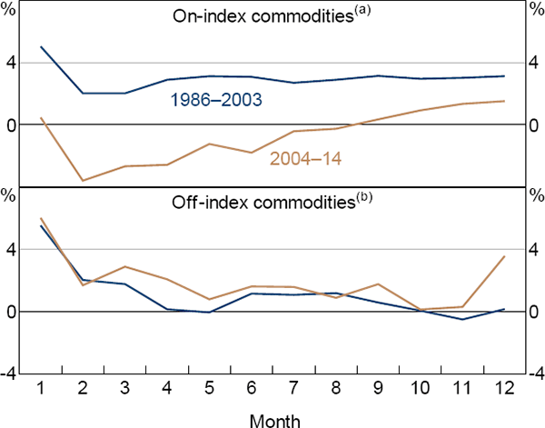
Notes: (a) Cattle, coffee, copper, corn, cotton, heating oil, hogs, natural gas, oil, soybeans, sugar, wheat (soft red wheat) (b) Lumber, milk, oats, orange juice, palladium, platinum, rice, soybean meal, wheat (Minnesota)
Sources: Authors' calculations; Pinnacle Data
To get a sense of the statistical significance of the above evidence, we can use a DD regression. This approach is essentially a more formalised statistical version of the graphical analysis above, which also allows us to incorporate control variables.[31] The regression compares the risk premiums for on-index commodities (treatment group) to off-index commodities (control group), both before and after the period of financialisation (treatment period). The post-financialisation period is again assumed to begin in 2004.
We consider three different DD models. Model 1 is the simplest. It is specified as:
where Indexc is a dummy that takes on the value one if the contract is for a commodity that is on-index (and is zero if off-index) and Post03t is a dummy that takes on the value one if the date is from 2004 onwards (and is zero before 2004).[32] Other terms are as defined in Equation (5).
This model focuses on changes in the residual risk premium. As such it can only be used to examine hypothesis 1, that financialisation has led to lower residual risk premiums. In testing this hypothesis we are interested in how the returns on on-index commodities changed relative to those on off-index commodities after financialisation (i.e. post-2003). This effect is captured by the coefficient, θ, which is known as the ‘difference-in-differences estimator’.
Model 2 extends the above model to better account for the systematic component of commodity risk premiums. The specification is:
where Marketm,t is the return on the market portfolio over horizon m. We use the MSCI All Country Weighted Index (MSCI) as the market portfolio as commodity markets are global and ergo a global index like the MSCI is likely to better represent the relevant market portfolio for speculators. The results obtained using a US equity index are similar.
We are trying to capture a few different concepts in this specification. As in Model 1, we are interested in how the average returns on on-index commodities changed relative to off-index commodities after financialisation, θ. As we now condition on the market portfolio's return, this should be a purer measure of the relative change in the residual risk premium.
We are also interested in how the betas of the on-index commodities changed relative to those of the off-index commodities after financialisation. This is captured by τ.[33] A positive significant estimate of τ would support hypothesis 2.
Finally, we wish to test whether the betas for on- and off-index commodities were different in the first period, which is captured by ϑ. If the betas for on- and off-index commodities differed, changes in the average market price of risk between the two periods will lead to relative changes in the systematic risk premiums for on- and off-index commodities. This would influence our estimates of θ and could lead to significant estimates of θ, even if financialisation had no influence. For example, take the beta for on-index commodities to be 0.8 and for off-index commodities to be 0.5 in the pre-financialisation period. A 1 percentage point rise in the market price of risk will cause the systematic risk premium for on-index commodities to rise by 0.8 percentage points and for off-index commodities to rise by 0.5 percentage points. As such, absent any effect from financialisation our estimate of θ would be 0.3 percentage points.
Both Models 1 and 2 treat the financialisation of commodities markets as a discrete event. In reality, it was a process that occurred (non-linearly) over a number of years starting in the mid 2000s.[34] Model 3 tries to account for this by incorporating separate financialisation dummies for each year into Model 2. More specifically:
where 1(Year = y)t is a dummy that equals one if the year is equal to y (and zero otherwise). We include dummies from 2001 onwards to allow for the possibility that financialisation began before 2004. Again, we are interested in how the returns for on-index commodities changed relative to those for off-index commodities after financialisation, which is captured by θt.[35]
Table 4 contains the results from Models 1 and 2. For Model 1, the average annualised returns declined by 2.6 percentage points more for on-index commodities relative to off-index commodities. While the sign of the coefficient is consistent with the first hypothesis, the coefficient is not statistically significant. To give some sense of the economic significance, the average annualised return for the full period was 2 per cent.
| Model 1 | Model 2 | |
|---|---|---|
| Financialisation dummy – θ | −0.026 | −0.043 |
| (0.047) | (0.045) | |
| Financialisation systematic risk dummy – τ | 0.253* | |
| (0.136) | ||
| Controls | ||
| Index – β | 0.017 | 0.024 |
| (0.032) | (0.033) | |
| Post03 – γ | 0.005 | −0.015 |
| (0.055) | (0.049) | |
| Market * Index – ϑ | −0.115 | |
| (0.081) | ||
| Post03 * Market – ρ | 0.433*** | |
| (0.088) | ||
| NHP | −0.010** | −0.105** |
| (0.044) | (0.045) | |
|
Notes: *, ** and *** indicate significance at the 10, 5 and 1 per cent level, respectively; Thompson (2011) standard errors are in parentheses and are robust to serial correlation, cross-sectional correlation, common serially correlated shocks and heteroskedasticity |
||
For Model 2, the estimate of θ is slightly larger than that from the previous specification (Table 4). Nevertheless, it is not statistically significant. Moreover, there is no evidence that ϑ is significantly different from zero, suggesting that changes in the market price of risk are not confounding our results. Finally, the estimate of τ is positive and statistically significant at the 10 per cent level. This provides some evidence that the beta for on-index commodities rose by more post-financialisation, relative to the beta for off-index commodities. That is, the correlation between returns on on-index commodities and on the market portfolio rose by more, consistent with the second hypothesis. All else equal, this should have led to larger systematic risk premiums for on-index commodities.
As discussed above, the influence of financialisation could differ for premiums on short- and longer-maturity futures contracts. To examine this possibility we run a generalised version of Model 2 which allows the ‘differences’ to differ by maturity bucket.[36]
There is still little evidence that financialisation affected the residual portion of risk premiums (hypothesis 1), at least when considering all on- and off-index commodities (Figure 6, top panel). However, when we allow the effects to vary by maturity bucket there is more consistent evidence that financialisation led to a relative increase in betas for on-index commodities (hypothesis 2). This is evident for contracts with maturities of around 6–12 months (Figure 6, bottom panel). This finding is somewhat consistent with Büyükşahin et al (2008), which found evidence of greater integration between prices for longer-term oil futures contracts post-financialisation, suggesting decreased segmentation in the markets for these contracts.
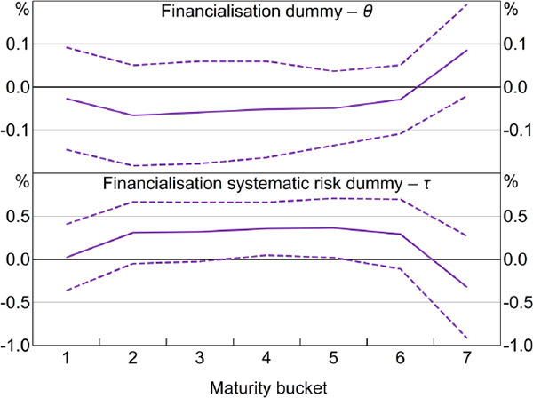
Note: Dashed lines are 95 per cent confidence intervals using errors robust to cross-sectional correlation, serial correlation and common serially correlated shocks
Figure 7 contains the results of Model 3. Returns generally decreased more for on-index commodities than for off-index commodities from around 2006 onwards. This suggests that our earlier findings that the effects of financialisation on average idiosyncratic risk premiums were not significant, in part, could reflect our choice of 2004 as the start of the financialisation period. Nevertheless, as discussed in Section 3.1, the use of ex post returns as a measure of risk premiums relies on the assumption of unbiased expectations. This is very unlikely to hold over periods as short as one year, so these results must be interpreted with caution.
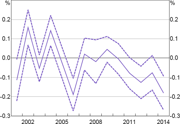
Note: Dashed lines are 95 per cent confidence intervals using errors robust to cross-sectional correlation, serial correlation and common serially correlated shocks
5.2 Commodity Case Studies
A concern with the above approach is that it conflates important variation between commodities in their supply and demand dynamics by imposing a common financialisation effect. This could make it difficult to find a statistically significant effect of financialisation, especially given the on- and off-index baskets are made up of somewhat different commodities. Relatedly, the DD approach assumes that the returns for on-index and off-index commodities would have followed the same time trends if financialisation had not occurred. This is somewhat hard to justify for baskets made up of different commodities.
Another approach that potentially ameliorates these concerns it to look at specific commodities. There are a number of examples where a commodity is included in, added to, or removed from an index while another similar commodity is not. We focus on two cases:
- Hard red wheat (HRW; GSCI only) and soft red wheat (SRW) are included in commodity indices while Minnesota wheat is not.
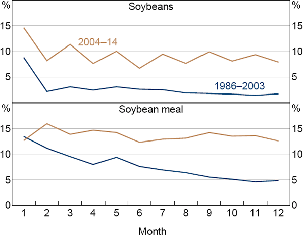
- Soybean oil (BCOM only) and soybeans are included in commodity indices while soymeal is only added in 2013. The validity of this case is somewhat more questionable, as soymeal is a by-product of the soybean oil production process and is used mainly as stock feed, rather than for human consumption. Nevertheless, it is worth considering.
Average risk premiums for SRW decreased in the post-financialisation period and this was more evident at the short end of the curve, with premiums falling by around 5 percentage points (Figure 8). In contrast, risk premiums for Minnesota wheat rose by around 5 percentage points along the curve. This difference is consistent with hypothesis 1. Meanwhile, risk premiums for both soybeans and soymeal rose by 5–10 percentage points in the financialised period (Figure 9).
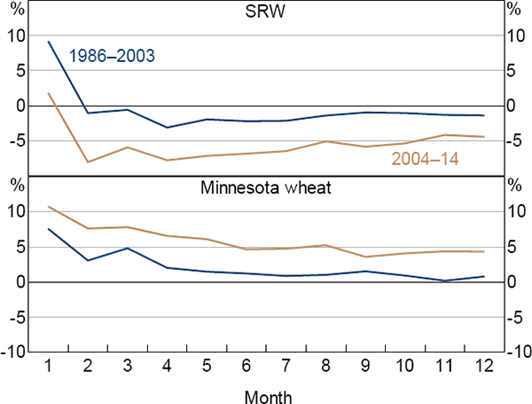
Sources: Authors' calculations; Pinnacle Data
Sources: Authors' calculations; Pinnacle Data
We can examine these cases more formally using a similar set-up to above, but using only the relevant commodities: SRW, HRW and Minnesota wheat; and soybeans, soybean oil and soymeal. For the latter we end the sample in 2012 (as soymeal was added to an index in 2013). We focus only on Models 1 and 2, due to the smaller number of observations.
Table 5 contains the results for wheat and soybeans. For Model 1, the estimates of θ are not statistically significant for both wheat and soybeans.
| Wheat | Soybeans | |||
|---|---|---|---|---|
| Model 1 | Model 2 | Model 1 | Model 2 | |
| Financialisation dummy – θ | −0.107 | −0.141* | 0.025 | 0.022 |
| (0.086) | (0.080) | (0.068) | (0.065) | |
| Financialisation systematic risk dummy – τ | 0.699** | 0.195** | ||
| (0.276) | (0.082) | |||
| Controls | ||||
| Index – β | 0.062 | 0.067 | −0.073** | −0.067* |
| (0.067) | (0.063) | (0.033) | (0.034) | |
| Post03 – γ | 0.052 | −0.049 | 0.038 | 0.017 |
| (0.100) | (0.108) | (0.075) | (0.086) | |
| Market * Index – ϑ | −0.074 | −0.116 | ||
| (0.203) | (0.095) | |||
| Post03 * Market – ρ | 0.130 | 0.485*** | ||
| (0.265) | (0.153) | |||
| NHP | −0.037 | −0.020 | 0.055 | 0.005 |
| (0.207) | (0.217) | (0.094) | (0.090) | |
|
Notes: *, ** and *** indicate significance at the 10, 5 and 1 per cent level, respectively; Thompson (2011) standard errors are in parentheses and are robust to serial correlation, cross-sectional correlation, common serially correlated shocks and heteroskedasticity |
||||
The estimate of θ is not significant for soybeans in Model 2. In contrast, there is some weak evidence that returns for on-index wheat contracts (HRW and SRW) declined more post-financialisation than those for off-index wheat. The decline of around 15 percentage points is economically significant, as average returns for SRW for the full sample were −2 per cent. Meanwhile, the estimate of τ is positive and significant for both wheat and soybean, suggesting that the beta for on-index wheat and soybean contracts increased, relative to those for off-index wheat and soybean contracts. All else equal, this should have increased the systematic portion of risk premiums.
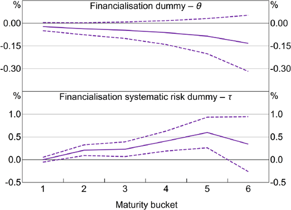
Again, we can estimate a generalised version of Model 2 that allows the effects to differ by maturity bucket. Due to the smaller number of observations and larger number of coefficients to be estimated, less general standard errors were used, so some caution must be taken in interpreting the results. For wheat, there is again evidence of a relative fall in returns for financialised wheat (at the 10 per cent significance level; Figure 10). Moreover, this evidence is generally stronger for short-maturity contracts. There is also evidence of relative increases in betas. The evidence is stronger for longer-maturity contracts, consistent with the above findings for a broad basket of commodities.
For soybeans (not shown), there is again little evidence of a relative change in returns for on- and off-index commodities. There is also evidence of relative increases in betas for longer-maturity contracts.
Note: Dashed lines are 95 per cent confidence intervals using errors robust to serial correlation
Footnotes
If we were able to model absolute risk premiums we could potentially differentiate. However, this cannot be done using ex post returns as a proxy for risk premiums, due to non-linearities in the absolute value transformation. [29]
The results are relatively robust to the choice of year to split the sample. Choosing a later year tends to lead to slightly more evidence that financialisation has affected risk premiums. [30]
Tang and Xiong (2012) use a similar set-up to consider whether financialisation caused prices for on-index commodities to become more correlated with oil prices. [31]
Results are broadly robust to including time dummies and contract-specific fixed effects, excluding NHP and allowing the coefficient on NHP to differ by maturity bucket. [32]
Another approach would be to construct a time-varying estimate of the betas for each contract by regressing commodity futures returns on the returns on the market portfolio over rolling windows, similar to Ferson and Harvey (1991). However, this approach was not compatible with the periodic nature of our data (see Appendix C). [33]
Tang and Xiong (2012) account for this by including a linear trend for the post-financialisation period. We prefer a method which imposes less structure on the progression of financialisation, particularly given the degree of financialisation appears to have peaked in around 2012 (at least in terms of AUM; Figure 3). [34]
We did not allow the relative change in the betas to vary by year, as this would entail a very large number of parameters. Moreover, our estimates of beta would be very noisy given the data are monthly. [35]
This is equivalent to stacking DD regressions for each separate bucket into one regression. [36]


