Research Discussion Paper – RDP2016-01 Measuring Economic Uncertainty and Its Effects
1. Introduction
Uncertainty has been a frequently cited reason for the weak global recovery from the financial crisis. This has been true for the United States, the European Union, and Australia (e.g. FOMC 2009; Balta, Valdés Fernández and Ruscher 2013; Kent 2014).
In this context, uncertainty refers to clarity, or lack thereof, about future economic activity. It incorporates both ‘risk’ and ‘Knightian uncertainty’. In the former, the probabilities of potential outcomes are known, but which outcome will occur is not. In the latter, neither the probabilities of outcomes nor the eventual outcome are known (Knight 1921; Cagliarini and Heath 2000). In practice, the two are difficult to disentangle, so I refer to a single concept of uncertainty that blends both in this paper.
Understanding economic uncertainty is difficult because it is not directly observable. In response, economists have developed a large and active literature that attempts to measure uncertainty and assess how heightened uncertainty affects the economy – both in theory and in practice.
In this paper I apply these techniques to Australia. To do so, I first review a number of commonly used proxies of uncertainty (Section 2). These proxies include: newspaper-based measures of uncertainty, like those created by Baker, Bloom and Davis (2015); finance-based measures, such as stock market volatility; and measures of disagreement among forecasters for key economic variables. Using some of these proxies, I construct a monthly index of economic uncertainty for Australia (Figure 5; Section 2.2).
I then use this index to document some stylised facts about uncertainty (Section 3). Uncertainty is estimated to be higher around some major geopolitical events, recessions, surprise changes in monetary policy, and federal elections. It also tends to increase more quickly than it decreases – spiking up rapidly around major events, and then fading more slowly. The index is also very persistent – periods of high or low uncertainty tend to last. Finally, both foreign and domestic factors appear to be relevant for uncertainty in Australia.
In Section 4, I use the index to assess how and why economic uncertainty might matter in Australia. There are reasons it should. First, under ‘real options’ theory, heightened uncertainty delays decisions that are costly to reverse (for instance, because of adjustment costs) because firms are better off waiting for uncertainty to subside before committing.[1] Second, heightened uncertainty may induce households to increase their precautionary savings and, therefore, reduce their consumption (Kimball 1990; Carroll 1997). In the short run, these responses are likely to be contractionary (Basu and Bundick 2012; Leduc and Liu 2015).
The Australian evidence is consistent with these theories: heightened uncertainty is estimated to weigh on economic activity. In particular, I find that employment growth slows modestly following a one standard deviation uncertainty shock, consistent with the real options channel of uncertainty. Also consistent with the real options channel, machinery and equipment investment growth slows in response to an uncertainty shock. The household saving ratio increases somewhat following an uncertainty shock and remains persistently elevated. This response is consistent with the precautionary savings channel of uncertainty.
2. Measuring Economic Uncertainty in Australia
Existing proxies for uncertainty fall into three broad categories: newspaper based; finance based; and forecaster disagreement. A brief survey of some other types of measures that have been used in the literature can be found in Appendix A.[2]
2.1 Measures of Economic Uncertainty
2.1.1 Newspaper-based measures[3]
To capture uncertainty reflected in media coverage, I follow Baker et al (2015) to construct a measure of newspaper articles that reference economic uncertainty.[4] The idea behind the measure is that information about economic uncertainty could be contained in newspaper coverage, not that media coverage causes economic uncertainty.[5]
These newspaper-based measures have a number of benefits. They capture a broad range of uncertainty (unlike, for example, finance-based measures) and are extremely timely – the search can be run daily, although I use monthly averages in this paper.
I collect data from four newspapers: The Australian; The Australian Financial Review (AFR); The Age; and The Sydney Morning Herald (SMH). Following Baker et al (2015), I search a database of newspaper articles (Factiva) for economic uncertainty-related articles. To meet the search criteria an article must contain ‘economy’ (or variants) and ‘uncertain’ (or variants) and at least one of the following terms: ‘budget’, ‘policy’, ‘legislation’ (or variants), ‘regulation’ (or variants), ‘parliament’, ‘senate’, ‘reserve bank’ or ‘RBA’. These restrictions are designed to exclude uncertainty-related articles that are not relevant to the economy and are similar to those used by Baker et al.
For each newspaper, I measure the number of articles that match the criteria relative to the total number of articles published in that month (Figure 1). The total number of articles used for the denominator includes all articles (e.g. current affairs, sports, lifestyle). The aggregate series is an equally weighted average of the individual newspaper measures.[6]
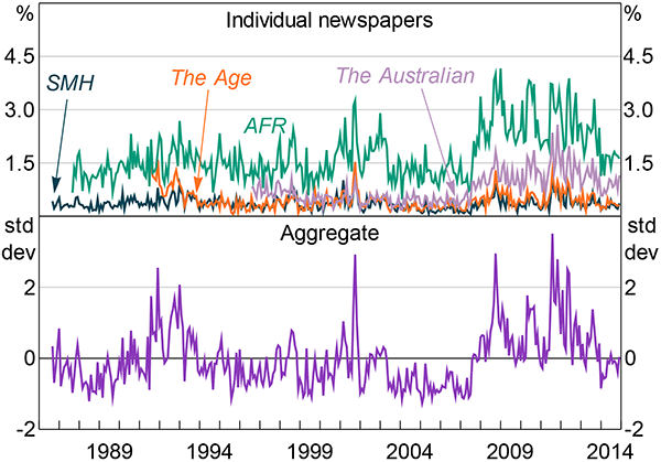
Note: The aggregate measure is an equally weighted average of the individual newspaper measures, which are first standardised to have mean 0 and standard deviation of 1 over August 1996 to December 2014
Sources: Author's calculations; Factiva
At first pass, the measures look sensible: they appear to capture major events fairly well, although they do often lag these events a little. For instance, the proportion of uncertainty-related articles in the AFR was higher in October 2008 than in September (when Lehman Brothers collapsed); the proportion in The Australian behaved similarly. These lags are partly a function of monthly averaging – Lehman Brothers collapsed in the middle of September, which means it would affect the totals for September less. But this behaviour also reflects the characteristics of the media coverage. In September, coverage focused on the immediate uncertainties for the US financial system and broad-sweeping articles about the crisis. By October, as the immediate turmoil subsided, coverage switched towards US and Australian government responses.
Consistent with the general theme of all the uncertainty proxies I review, the individual newspaper measures are highly correlated with one another (Table 1). The more business-focused newspapers – The Australian and the AFR – are most strongly correlated. These newspapers also have higher proportions of economic uncertainty-related articles, given their business focus.
| The Australian | AFR | The Age | SMH | Aggregate | |
|---|---|---|---|---|---|
| The Australian | 1 | ||||
| AFR | 0.76 | 1 | |||
| The Age | 0.62 | 0.69 | 1 | ||
| SMH | 0.51 | 0.57 | 0.76 | 1 | |
| Aggregate | 0.84 | 0.88 | 0.89 | 0.83 | 1 |
|
Notes: All correlations are significantly different from zero at the 1 per cent level; all correlations are for the period August 1996 to December 2014 because there are no data for The Australian prior to this date Sources: Author's calculations; Factiva |
|||||
There are methodological drawbacks to these types of measures. In particular, false positives are unavoidable. However, Baker et al (2015) used similar search terms for the United States and audited the results by reading through a large number of articles to check whether the articles were in fact about economic uncertainty. Although there were some differences between the machine-created and the hand-created series, the two series were strongly correlated. In addition, the error rates were uncorrelated with economic variables.
2.1.2 Finance-based measures
Stock market volatility is a commonly used proxy for uncertainty because it is available in real time and is reasonably comparable across countries. For example: Caggiano, Castelnuovo and Groshenny (2014) use it to assess the effects of uncertainty on the US economy; Bekaert, Hoerova and Lo Duca (2013) decompose it into a risk aversion component and an uncertainty component to test how monetary policy affects both; and Baker and Bloom (2013) use natural disasters and stock market volatility to assess the effects of uncertainty.
Realised volatility – measured here by the monthly average of the daily absolute percentage change in the All Ordinaries index – is one measure of stock volatility.[7] The main benefit of this measure of stock volatility is that it provides a very long time series. However, because uncertainty is necessarily about the future, forward-looking measures of stock volatility are conceptually preferable. A measure of forward-looking stock market volatility can be constructed from the implied volatility of call and put options on the ASX 200 index (Figure 2).[8] It represents the expected one-month-ahead volatility in the ASX 200. Unfortunately, data for option-implied volatility are more limited than some of the other measures I use in this paper – data are only available from 1995 – which means it does not cover, for example, the early 1990s recession.
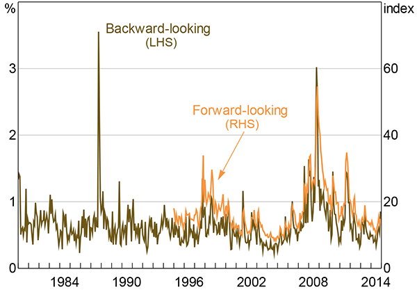
Notes: The forward-looking measure is the monthly average of daily option-implied volatility for the ASX 200; the backward-looking measure is the monthly average of the absolute value of daily percentage changes in the All Ordinaries index
Source: Thomson Reuters
The drawback of these stock volatility measures is that they are only indirectly connected to economic activity. Although company earnings are connected to economic activity, much of the short-run variation in stock prices is driven by other factors (Shiller 1981; Cochrane 2011). Although these factors may relate to economic uncertainty, the connection to economic activity is not clear. These measures are also asymmetric – increases in the measures accompany large falls in stock prices; large gains in stock prices are less common.
Another finance-based measure of uncertainty is the dispersion in analysts' forecasts for 12-month-forward earnings for ASX 200 companies. The benefit of this measure is that it is more directly connected to economic activity – corporate profits are part of GDP – than measures of stock volatility. It is also quite timely, although less so than stock volatility measures. However, it has a much shorter history than most other measures and, like other measures of forecaster disagreement, might capture disagreement, rather than uncertainty (this issue is discussed in Section 2.1.3).
The measure is calculated as the cross-sectional coefficient of variation of analysts' forecasts for each ASX 200 stock. This is then aggregated to obtain an average for all ASX 200 companies, and for sectors (Figure 3).
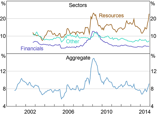
Note: Coefficient of variation on 12-month-forward earnings forecasts
Sources: MSCI; Thomson Reuters
2.1.3 Forecaster disagreement
Measures of dispersion between forecasters for economic variables can also proxy for economic uncertainty (Figure 4). Heightened economic uncertainty widens the potential distribution of outcomes; this should show up as greater dispersion among forecasters.
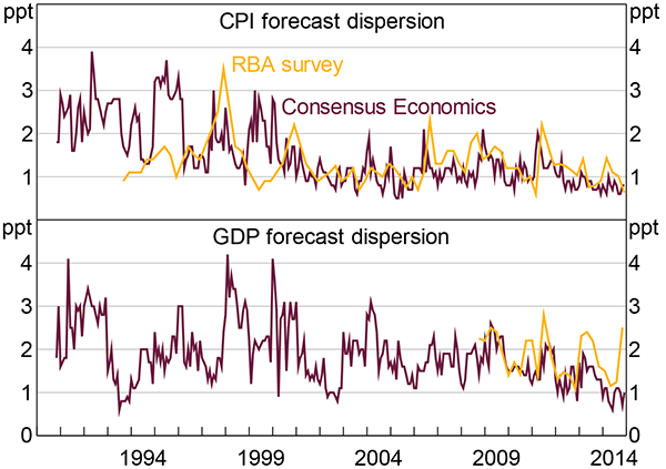
Notes: Range between highest and lowest forecast; Consensus Economics survey forecasts are for the next calendar year; RBA survey forecasts are for year-ended growth between four and five quarters ahead (depending on the date of the survey)
Sources: Author's calculations; Consensus Economics; RBA
However, an important criticism of measures of forecast dispersion is that forecast dispersion and uncertainty are not identical. Forecast dispersion might instead capture disagreement – how far forecasters are from one another – not uncertainty. Each forecaster could be extremely certain, but there could still be a high degree of disagreement (and vice versa). Some authors have argued that, in light of this distinction, forecast dispersion is a poor proxy for uncertainty (Rich, Song and Tracy 2012).
On the other hand, forecast dispersion measures are closely conceptually connected to economic activity. Moreover, these measures are timely – for instance, the Consensus Economics survey is typically conducted in the early part of the month and the responses are published shortly thereafter.
There is a reasonable degree of correlation between the different measures of forecast dispersion for which I have data, across both different surveys and different forecasted variables (Table 2). These correlations suggest that there is a common element that drives dispersion among forecasts for different economic variables.[9] There is also statistically significant correlation between the dispersion in cash rate forecasts and the dispersion in GDP forecasts, but not with the dispersion in CPI forecasts (Table 2).[10]
| RBA survey of market economists – CPI | RBA survey of market economists – GDP | Consensus Economics – CPI | Consensus Economics – GDP | Market economists' cash rate forecasts | |
|---|---|---|---|---|---|
| RBA survey of market economists – CPI | 1 | ||||
| RBA survey of market economists – GDP | 0.05 | 1 | |||
| Consensus Economics – CPI | 0.27** | 0.28 | 1 | ||
| Consensus Economics – GDP | 0.28** | 0.60*** | 0.35*** | 1 | |
| Market economists' cash rate forecasts | 0.33 | 0.41* | 0.05 | 0.43*** | 1 |
|
Notes: Range between highest and lowest forecast; Consensus Economics forecasts are for the next calendar year; RBA forecasts are for year-ended values between four and five quarters ahead (depending on the date of the survey); market economists' cash rate forecasts are for the level of the cash rate in two quarters time; ***, ** and * denote statistical significance at the 1, 5 and 10 per cent levels, respectively; pairwise correlations are for the maximum available period, based on data availability (see Appendix B for details on data availability by series); all correlations are at monthly frequency except RBA survey of market economists, which is against the quarterly average of the other series Sources: Author's calculations; Consensus Economics; RBA |
|||||
A drawback of these types of dispersion measures is that outlying observations can exert a large influence, and the measures I use – based on the range – are particularly susceptible. Single contrarian forecasts can cause large increases in the range, even if the rest of the forecasts are tightly clustered. This is more of an issue because the samples of forecasters are not constant in the surveys I use. For example, Consensus Economics surveyed a particularly contrarian forecaster during the early part of 2000 who consistently forecast GDP growth roughly 2 percentage points lower than the vast majority of other forecasters.[11] This forecaster was not included in all surveys. As a result, the Consensus Economics GDP forecast dispersion measure was very volatile in early 2000 as this forecaster transitioned in and out of the survey sample. Measures of dispersion that ignore outliers – such as the interquartile range – can mitigate these issues. Unfortunately, I do not have access to data for the interquartile range.
2.1.4 Correlations between the measures
Even if each of the measures reviewed above represents a noisy signal of some true underlying process of economic uncertainty, there should be a reasonably high degree of correlation between all these measures. Table 3 shows that this is the case.
| Option-implied volatility(a) | Realised volatility | Analyst earnings forecast uncertainty (ASX 200)(a) | Proportion of uncertainty-related articles (aggregate)(a) | SMP- based measure | RBA survey of market economists – CPI | Consensus Economics – GDP(a) | Consensus Economics – CPI | |
|---|---|---|---|---|---|---|---|---|
| Finance-based measures | ||||||||
| Option-implied volatility(a) | 1 | |||||||
| Realised volatility | 0.85*** | 1 | ||||||
| Analyst earnings forecast uncertainty (ASX 200)(a) | 0.66*** | 0.45*** | 1 | |||||
| Text-based measures | ||||||||
| Proportion of uncertainty-related articles (aggregate)(a) | 0.59*** | 0.38*** | 0.45*** | 1 | ||||
| SMP-based measure | 0.05 | −0.02 | 0.09 | 0.34*** | 1 | |||
| Forecast dispersion | ||||||||
| RBA survey of market economists – CPI | 0.29** | 0.25** | 0.31** | 0.04 | −0.11 | 1 | ||
| Consensus Economics – GDP(a) | 0.11* | −0.04 | 0.13* | −0.03 | −0.03 | 0.28** | 1 | |
| Consensus Economics – CPI | 0.11* | −0.03 | 0.33*** | 0.00 | −0.01 | 0.27** | 0.35*** | 1 |
|
Notes: ***, ** and * denote statistical significance at the 1, 5 and 10 per
cent levels, respectively; pairwise correlations are for the maximum
available period, depending on data availability (see Appendix B for details on data
availability by series); all correlations are at monthly frequency except
RBA survey of market economists and the Statement on Monetary
Policy (SMP)-based measure, which are against the
quarterly average of the other series; measures with limited data are
excluded from this table Sources: Author's calculations; Consensus Economics; Factiva; MSCI; RBA; Thomson Reuters |
||||||||
The main exception is that all three measures of forecast dispersion in Table 3 are only modestly correlated with the finance-based measures of uncertainty and are uncorrelated with the newspaper-based measure. This low degree of correlation might reflect the effects of adverse shocks that reduce expected growth in ways that do not increase forecast dispersion – i.e. because forecasters agree on the likely outcome – but which are still associated with increases in uncertainty that are picked up by the other proxies. This issue of forecaster disagreement versus uncertainty is discussed in Section 2.1.3.
2.2 An Index of Economic Uncertainty for Australia
All the measures co-move and behave similarly around major events. These facts suggest that there is some underlying ‘economic uncertainty’ process. I use four of the measures to construct a monthly economic uncertainty index for Australia (Figure 5). The index tries to capture this underlying process by smoothing away the noise inherent in any particular measure. The components of the index are: economic uncertainty-related newspaper articles; forward-looking stock market volatility; analyst earnings forecast uncertainty; and GDP growth forecast dispersion.[12] I use these components because they are timely and capture a broad range across the three categories of uncertainty measures.
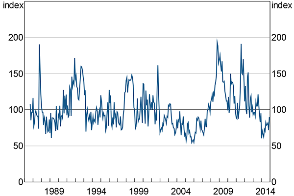
Note: For the period November 2000 to December 2014: mean = 100 points, standard deviation = 30 points
Sources: Author's calculations; Consensus Economics; Factiva; MSCI; Thomson Reuters
The index is a weighted average of the standardised components. The weights are: 50 per cent on the newspaper-based measure; one-sixth on each of the remaining three measures. I use these weights because they match those used by Baker et al (2015). Appendix C shows that the index is robust to different weights. This is unsurprising given the correlation among the measures.
I scale the index so that it has mean of 100 points and standard deviation of 30 points over the period November 2000 to December 2014. This choice is arbitrary; I pick these figures for the mean and standard deviation because they are similar to the headline index from Baker et al (2015). Over the full history, the index has a mean of 101 points and a standard deviation of 27.5 points.[13] Appendix C explains how the index is constructed and how I deal with changes in data availability over time.
Like the indices from Baker et al (2015), the index captures economic policy uncertainty through the newspaper-based component.[14] Indeed, the uncertainty-related news articles component from Section 2.1.1 is an analogue of the many country-specific economic policy uncertainty indices from Baker et al (2015). However, the index I construct captures a broader range of economic uncertainty than Baker et al's economic policy uncertainty indices because of the other components I include. In particular, I use stock market volatility and analyst earnings forecast uncertainty in place of upcoming tax code expirations and forecast dispersion for government purchases of goods and services. Comparable data for Australia do not exist for these components.
Late 2014 is a good example of the conceptual distinction between economic uncertainty and economic policy uncertainty, and why I aim for the broader concept. In late 2014, the outlook for China became more uncertain, which was associated with falling commodity prices. This type of uncertainty is likely relevant for the Australian economy, and so an index of uncertainty ideally should capture it. However, it is not the result of policy decisions by Australian agencies; indeed, the newspaper-based measure did not move around this time. Rather, the analyst earnings forecast uncertainty measure picked up this event.
3. Stylised Facts about Uncertainty
This section uses the economic uncertainty index to understand the dynamics of economic uncertainty and document some stylised facts. In Section 3.1 I argue that the index passes the first sense test: it lines up with major events that might be expected to correspond to high uncertainty. In Section 3.2 I show that, although many of the major events from Section 3.1 are foreign, there is still a substantial amount of domestic variation in the index. Having established these properties, in Section 3.3 I document some statistical properties of the index. Finally, in Sections 3.4 to 3.6 I show that the index correlates with Australian recessions, elections and monetary policy decisions.
Appendix D contains some further stylised facts, including how the economic uncertainty index relates to measures of consumer or business sentiment.
3.1 Major Events
The index lines up with events that a priori might be expected to create economic uncertainty (Table 4; Figure 6). This fact is reassuring because it suggests the index is indeed capturing uncertainty.
| Date | Event | Uncertainty index | Change from previous month |
|---|---|---|---|
| 20 October 1987 | (A) Black Monday (19 October in the United States) | 190 | +117 |
| 29 November 1990 | (B) ‘Recession we had to have’ speech – approximate start of the Australian early 1990s recession | 101 | −19 |
| November 1992 | (C) Australian unemployment peaks at 11.1 per cent | 155 | −4 |
| 2 July 1997 | (D) Baht floated – beginning of Asian financial crisis | 73 | +1 |
| 17 August 1998 | (E) Russian Federation defaults | 142 | +2 |
| 23 September 1998 | (F) Long-term Capital Management collapses | 148 | +5 |
| 11 September 2001 | (G) 9/11 terrorist attacks | 132 | +47 |
| 20 March 2003 | (H) US invasion of Iraq | 108 | +4 |
| 14 March 2008 | (I) Bear Sterns rescued | 120 | +6 |
| 15 September 2008 | (J) Lehman Brothers files for Chapter 11 bankruptcy protection | 148 | +9 |
| 23 April 2010 | (K) Greece requests official financial assistance | 102 | +6 |
| 31 July 2011 | (L) US debt ceiling stand-off – the debt ceiling is raised days before it would have been reached in August | 132 | +27 |
| 9 March 2012 | (M) Greek debt restructuring becomes effective | 100 | −33 |
|
Sources: Author's calculations; Consensus Economics; Factiva; MSCI; Thomson Reuters |
|||
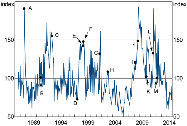
Notes: See note to Figure 5; see Table 4 for label definitions
Sources: Author's calculations; Consensus Economics; Factiva; MSCI; Thomson Reuters
Some of the events do not induce large in-month increases, but subsequent months have relatively large increases. Sometimes this is because the events occur late in the month – such as Greece requesting financial assistance in April 2010 – and so most of the increase occurs in the succeeding month. For some other events, uncertainty simply seems to respond more slowly – the 9/11 attacks induced a sizeable and rapid increase in uncertainty; the start of the Asian financial crisis induced a slower response. Some events correspond to decreases in the index because they resolve uncertainty; the Greek debt restructuring in March 2012 is a good example. Not all geopolitical events correlate with high estimated uncertainty; the index was not elevated around the US invasion of Iraq in March 2003.
3.2 Foreign and Domestic Uncertainty
As a small open economy, foreign economic shocks can have a large effect on Australia. Uncertainty is no exception – a number of major international events correspond to sizeable spikes in estimated uncertainty (Table 4, Section 3.1). However, regressing the economic policy uncertainty index for the United States from Baker et al (2015) on the Australian index accounts for less than a third of the overall variation in the Australian index (Figure 7). Foreign events such as the 9/11 attacks and the 2011 US debt ceiling stand-off are largely explained by the foreign component: the blue (Australian) and pink (US predicted) series line up. But most of the month-to-month variation in the index cannot be explained by foreign factors.
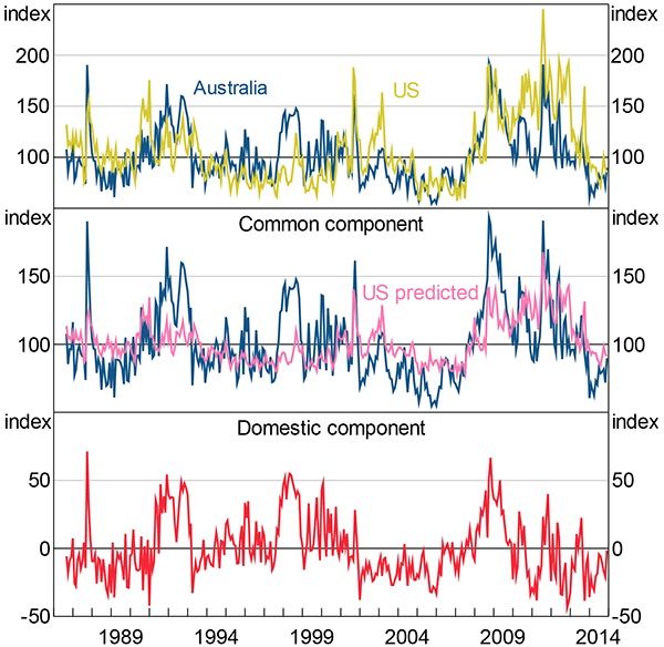
Notes: See note to Figure 5; the ‘US predicted’ series is from a regression of the Australian economic uncertainty index on the US economic policy uncertainty index from Baker et al (2015); ‘domestic component’ is the residual from that regression
Sources: Author's calculations; Baker et al (2015); Consensus Economics; Factiva; MSCI; Thomson Reuters
Foreign uncertainty seems to have been higher than domestic uncertainty since the global financial crisis. The two indices both increased rapidly during the early stages of the global financial crisis (top panel, Figure 7). However, the Australian index declined sooner. Indeed, the domestic component has never exceeded 30 points since the end of 2011.
3.3 Uncertainty Increases Faster than It Decreases
The business cycle is generally thought of as asymmetric – output grows in a relatively steady manner during expansions, but falls sharply during recessions. These types of dynamics are easily observed in the unemployment rate, but many have argued these dynamics are more general.[15]
The uncertainty index appears to be similar – increases in the economic uncertainty index tend to be larger than decreases. The distribution of changes in the index is positively skewed, with a skewness coefficient of 0.8. It is also fat-tailed, with excess kurtosis of 4.4. The distribution is significantly different from the normal distribution.[16]
Similarly, periods of high or low uncertainty tend to persist. The one-period autocorrelation of the index is 0.76 and the second-lag partial autocorrelation is 0.20. Further lags are not significantly different from zero. Despite the high degree of persistence, the economic uncertainty index is stationary – even with 12 lags, the p-value for the augmented Dickey-Fuller test is just 0.02.
Taken with Table 4, these facts suggest that the dynamics of uncertainty are often characterised by large spikes upward after major events, followed by slow reversion.
3.4 Recessions
Bloom (2014) shows that, for the United States, uncertainty is higher during recessions. In Australia, there have been few recessions during the period for which data exist for the economic uncertainty index. This makes it difficult to assess the relationship between uncertainty and recessions.
Nonetheless, there is some evidence that uncertainty is higher when unemployment is rising (Figure 8). The economic uncertainty index is on average 20 points higher in months where the unemployment rate is trending upwards than in months where it is trending downwards. In addition, trend employment growth and seasonally adjusted GDP growth are negatively correlated with the economic uncertainty index; however, the correlation is much weaker for GDP.
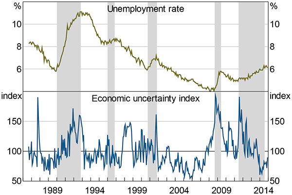
Notes: See note to Figure 5; shaded areas show periods where the unemployment rate is trending upwards; turning points are (somewhat arbitrarily) identified as the last minimum and the first maximum
Sources: ABS; Author's calculations; Consensus Economics; Factiva; MSCI; Thomson Reuters
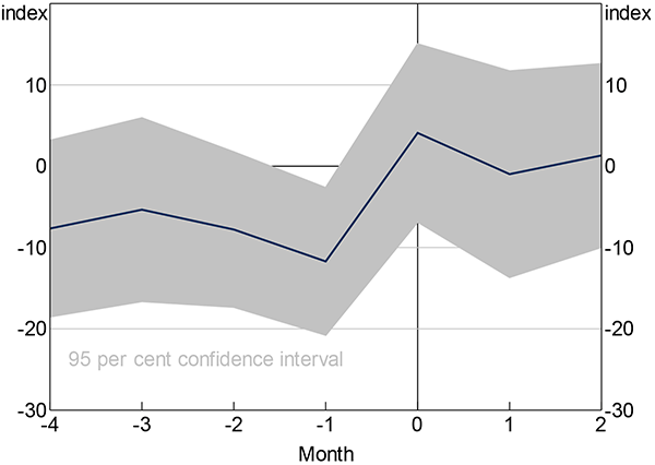
3.5 Federal Elections
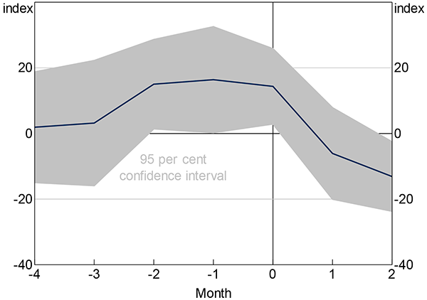
Federal elections are an opportunity to isolate a domestic event. Federal elections may elevate uncertainty because of uncertainty about the outcome of the election and the potential for changes to government policies. I test whether this is true by regressing the economic uncertainty index on dummy variables for near-election months. The coefficients represent the average in-month level of the index, relative to its remaining history. I have not controlled for any other relevant factors.[17]
Economic uncertainty is estimated to be higher than average before federal elections and in the month of the election (Figure 9). In the two months leading up to the election and the month of the election, the economic uncertainty index is 14 to 16 points higher than average, depending on the month.[18] This lines up with approximately when campaigning would begin to increase. As expected, estimated economic uncertainty declines following elections.
Sources: Author's calculations; Consensus Economics; Factiva; MSCI; Thomson Reuters
However, Figure 9 masks a lot of dispersion: both the 2010 Federal election (which resulted in a hung parliament) and the 1998 Federal election coincided with in-month index levels of around 140; the 2004 election had an economic uncertainty index level of 91 points. The uncertainty around elections is probably related to how close the election result is. I do not take this into account here, but further work could examine whether closer elections – perhaps measured by poll results – align with higher economic uncertainty.
3.6 Monetary Policy Decisions
The RBA's monetary policy decisions are another set of domestic events which could be related to economic uncertainty. Changes in monetary policy that are not generally expected might be related to economic uncertainty either because: unexpected changes in monetary policy cause uncertainty (for instance, by making firms' financing decisions less certain); or, when economic uncertainty is higher, it might be harder for market participants and commentators to predict the path of monetary policy (and other economic aggregates).
I measure ‘monetary policy surprises’ by the absolute difference between the market-implied cash rate the day before a cash rate decision and the subsequent decision. These surprises capture both unexpected movements and anticipated movements that occur earlier or later than expected.
The economic uncertainty index is indeed correlated with ‘monetary policy surprises’ (Figure 10). The two series have a correlation coefficient of 0.49, which is statistically significant at the 1 per cent level, despite the fact that I only have market-implied cash rate data going back to February 2005. Of course, these correlations cannot disentangle which way causality flows between uncertainty and monetary policy.
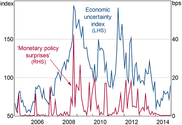
Notes: See note to Figure 5; ‘monetary policy surprises’ are measured by the absolute difference between the overnight indexed swap-implied cash rate at market close the day before the RBA Board meeting and the actual cash rate decision
Sources: Author's calculations; Consensus Economics; Factiva; MSCI; RBA; Thomson Reuters
4. The Effects of Uncertainty on the Australian Economy
In this section, I examine whether and how uncertainty matters for the Australian economy. I do so by estimating two vector autoregressions (VARs) – one at monthly frequency and one at quarterly frequency.
Theory predicts that heightened uncertainty should delay decisions that are costly to reverse – such as hiring and investment. Once uncertainty subsides, businesses should then catch up on these delayed decisions, leading to overshooting. This is the ‘real options’ channel of uncertainty (Bernanke 1983; Dixit and Pindyck 1994; Bloom 2009).[19] If the theory is valid, we should see initial falls in investment and employment growth in response to an unexpected increase in uncertainty, followed by growth, then overshooting. The precautionary savings channel of uncertainty predicts that the household saving ratio should rise and that consumption growth – particularly discretionary consumption – should fall following a rise in uncertainty (Kimball 1990; Carrol 1997).
4.1 Monthly VAR
In this section I test the real options channel of uncertainty on employment. Because labour force data directly address the real options channel for employment and are available monthly, I use a monthly VAR. This allows me to exploit the monthly variation in the uncertainty index. In addition to uncertainty and employment, I include three other relevant economic series that are also available monthly: retail sales growth; the cash rate; and ANZ-Roy Morgan consumer confidence.[20]
I use one lag in the VAR. The results appear to be robust to using one, two or three lags; I choose to use one for parsimony. Appendix E.1 shows results from alternative specifications.[21]
I use a Cholesky decomposition with the economic uncertainty index ordered last. This assumption imposes the restriction that shocks to the other economic variables affect the economic uncertainty index contemporaneously, but uncertainty only affects other variables with a lag. This is a conservative identification assumption. By ordering the economic uncertainty index last, the identified uncertainty shocks are purged of any predictable component due to any of the other variables. For sentiment in particular, this can be material. As a result, this assumption will tend to reduce the size of the estimated responses compared to alternative orderings. For this reason, the estimates can be thought of as representing a lower bound.
Much of the empirical literature takes the opposite approach and orders uncertainty first. Because of this, I also present estimates that have the economic uncertainty index ordered first (Appendix E.2). The effects of uncertainty are larger with this identification assumption, but the difference is generally not large and the qualitative results are unchanged. Since the more-conservative assumptions are enough to show that uncertainty matters, I use these in the main text.
The estimated effects of a one standard deviation (30 point) shock to the economic uncertainty index on economic activity are shown in Figure 11. The key result is that employment growth is persistently lower. However, the peak effect is only modestly sized – annualised monthly employment growth declines by about one-sixth of a percentage point after four months. For comparison, average annualised monthly employment growth over the period is 1.8 per cent. The response is statistically different from zero for four months (at the 5 per cent level, between six and nine months after the shock), but the confidence intervals are wide and an initial increase in growth is comfortably within the confidence interval. This response provides support for the real options channel. In contrast to real options theory, I find no evidence of overshooting as firms catch up on hiring decisions that were delayed by uncertainty; however, there is a deal of uncertainty around more-distant estimates, and I cannot reject an increase in growth after ten months.
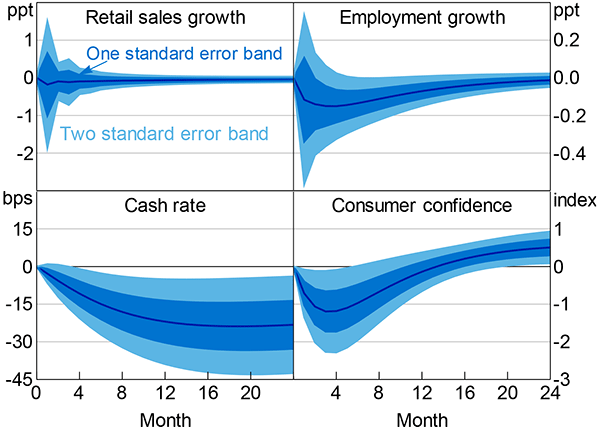
Notes: Retail sales growth and employment growth are annualised; estimation covers October 1986 to December 2014
Retail sales growth decreases, but the magnitude is small – annualised monthly growth is reduced by about one-sixth of a percentage point, compared to average annualised monthly growth of about 5 per cent. The confidence intervals are wide and include a large mass above zero. This response therefore provides little evidence in support of a precautionary savings channel, which predicts that consumption growth should be lower. However, retail sales growth is not a complete measure of consumption and it is also a relatively poor measure of discretionary consumption, which the precautionary savings channel predicts should be most affected.[22] I examine the precautionary savings channel with better-suited quarterly data in Section 4.2. Consequently, I place little weight on the precautionary savings evidence from the monthly VAR.
Uncertainty shocks are estimated to have a small effect on consumer confidence. Following an uncertainty shock, consumer confidence decreases by 1.2 points after three months, although it is slightly positive after a little over a year, before returning to baseline. This initial decrease equates to a little less than a tenth of a standard deviation. The small magnitude of this change is reassuring – it suggests that the responses do reflect uncertainty shocks, not combined sentiment and uncertainty shocks.
Uncertainty shocks have a noticeable effect on the level of the cash rate, which decreases by a little less than a quarter of a percentage point within a year after the shock. Monetary policy is potentially responding to the likely effects of uncertainty on other relevant macroeconomic variables. Such a response of the cash rate might help mitigate the effects of uncertainty on employment somewhat.
4.1.1 Does foreign or domestic uncertainty matter?
As noted in Section 3.2, foreign uncertainty appears to be an important source of uncertainty for Australia. As a small open economy, this is unsurprising. In this light, it is possible that foreign uncertainty shocks affect economic outcomes differently than domestic shocks.
I test this hypothesis by using the US economic policy uncertainty index from Baker et al (2015) to separate foreign and domestic uncertainty shocks (Figure 12).[23] I do so by ordering the US index ahead of the Australian index in the monthly VAR and restricting the response of the US index such that it does not respond to any of the Australian variables; all Australian variables are able to respond to shocks to the US index.[24]
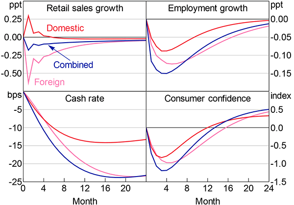
Notes: Retail sales growth and employment growth are annualised; the ‘combined’ series shows the same responses as Figure 11 for comparison; estimation covers October 1986 to December 2014
It appears that domestic and foreign shocks have similar effects (Figure 12). Although the foreign shocks appear to have a marginally larger effect, these responses are not precisely estimated and the confidence intervals are wide. In sum, these results suggest that foreign and domestic uncertainty shocks affect Australian economic outcomes similarly. It is uncertainty that matters, not the source of uncertainty. In the quarterly VAR I do not distinguish between foreign and domestic uncertainty shocks.
4.2 Quarterly VAR
I test for evidence of the precautionary savings and real options (investment) channels using a quarterly VAR that incorporates eight data series: growth in machinery and equipment (M&E) investment; growth in household final consumption expenditure on durable goods; growth in employment; the household saving ratio; changes in the terms of trade; the quarterly average of the cash rate; the quarterly average of ANZ-Roy Morgan consumer sentiment; and the quarterly average of the economic uncertainty index.
For the reasons discussed in Section 4.1, I again adopt a conservative identification strategy by using a Cholesky decomposition with the economic uncertainty index ordered last. As with the monthly VAR, Appendix E.4 shows that ordering the economic uncertainty index first increases the responses, but the difference is not substantial and the overall story is unchanged.
I estimate a VAR with two lags.[25] The results are robust to other lag specifications and orderings, with the exception of using one lag with the economic uncertainty index ordered last (Appendix E.5).
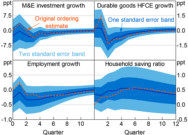
Consistent with the predictions of the real options channel of uncertainty, M&E investment growth decreases and remains persistently weaker following a one standard deviation uncertainty shock (Figure 13); however, the confidence intervals are wide and cover a large mass above zero. The peak magnitude of the reduction (after three quarters) in annualised quarterly growth is a little less than 4 percentage points; this response compares to average annualised quarterly M&E investment growth of a little less than 7 per cent.[26] However, as with the monthly results from Figure 11, I find no evidence of overshooting.
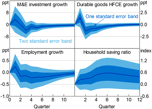
Notes: Machinery and equipment (M&E) investment growth, durable goods household final consumption expenditure (HFCE) growth and employment growth are annualised; omitted responses are in Figure E3; estimation covers June quarter 1987 to December quarter 2014
The initial increase in growth in the quarter following the shock is surprising, and is followed by a sharp reversal and more persistent reduction in growth. Ordering the economic uncertainty index ahead of consumer sentiment (or first) largely eliminates this initial spike (Appendix E).
The results support the precautionary savings channel: the household saving ratio rises by just more than half a percentage point and remains persistently elevated. This increase is not insubstantial relative to the average household saving ratio of around 5½ per cent over the sample period. Also consistent with the precautionary savings channel of uncertainty, annualised quarterly growth in the consumption of durable goods falls by as much as 1.3 percentage points.[27] This reduction compares to average annualised quarterly growth of a bit more than 3 per cent. As with the saving ratio, this is a not insubstantial effect and lends reasonable support to the precautionary savings channel.
In terms of the other responses from the quarterly VAR, employment growth appears broadly similar to the response in Figure 11. Reassuringly, the reduction in (annualised quarterly) growth between two to eight quarters (inclusive) is between about 0.15 to 0.20 percentage points, which is a little larger than the roughly one-sixth of a percentage point response estimated at monthly frequency around months two through six. The response in the quarterly VAR is also much more persistent – in the monthly VAR the effect has largely dissipated after two years, but in the quarterly VAR the response is estimated to be a little over 0.1 percentage points at the same point. As noted for investment growth, the initial increase in employment growth is surprising in light of both theory and the subsequent persistent reduction. The response of consumer confidence and the cash rate are similar to those estimated in the monthly VAR, although a little smaller. The terms of trade barely respond to an uncertainty shock. For more detail see Appendix E.3.
4.3 Comparison to Other Literature
There is a large empirical literature that attempts to assess the effects of uncertainty shocks; the vast majority of it focuses on the United States.[28] My estimates of the effects of uncertainty are generally a little smaller.
Based on a similar aggregate-level VAR framework, Bloom (2009) finds that uncertainty shocks lead to a 1 per cent decrease in industrial production and about a 0.7 per cent decrease in employment. In a similar vein, Caggiano et al (2014) use a smooth transition VAR – which allows them to differentiate between recessions and expansions – and find that an uncertainty shock raises the unemployment rate about 0.17 percentage points four quarters after the shock. During a recession, the effect is larger – about 0.36 percentage points. They also find the level of investment falls about 3 per cent below trend during a recession in response to an uncertainty shock. They argue that distinguishing between uncertainty shocks in recessionary and non-recessionary phases is important.[29]
Bloom et al (2013) use a calibrated macroeconomic model to study the effects of uncertainty on economic activity. They find that uncertainty shocks decrease the level of GDP by about 2 per cent below trend, and hours worked by about 2.5 per cent. The decrease they find is larger, occurs much faster, and is less persistent than what I estimate for employment. In a similar vein, Leduc and Liu (2015) use a macroeconomic model with search frictions and nominal rigidities. They find that an uncertainty shock increases the unemployment rate by about 0.15 percentage points at peak (after about 18 months). This result is a little larger than what my estimates for employment growth imply for the unemployment rate. In contrast, Bachmann and Bayer (2011) argue that uncertainty shocks are only a small driver of fluctuations in economic activity.
Carriero et al (2015) argue that the measurement error inherent in proxies for uncertainty can substantially attenuate the estimated impulse responses, but using the uncertainty proxy as an instrument eliminates the bias. They apply their method to the dataset from Bloom (2009) and find substantially larger effects from uncertainty than Bloom. These results suggest that my estimates may understate the effect of uncertainty.
In terms of Australian studies, Tran (2014) uses firm-level data on investment and both firm- and aggregate-level measures of uncertainty to assess how uncertainty affects investment. The results suggest that uncertainty weighs on investment, and that firm-specific uncertainty is more relevant than aggregate-level uncertainty.
Other Australian macroeconomic VARs have tended to focus on identifying monetary policy shocks. These include Berkelmans (2005), Lawson and Rees (2008) and Dungey and Pagan (2009) among others. A possible extension of my work is to examine how uncertainty might affect the results of those papers, particularly given that Caggiano et al (2014) find asymmetric effects of uncertainty during recessions.
5. Conclusion
A newly constructed monthly economic uncertainty index lines up well with events that would be expected to increase uncertainty and with other proxies of economic uncertainty. Based on the index, economic uncertainty rose to historically high levels during the global financial crisis and remained above long-term average until late 2013. It was a bit below average for all of 2014.
I use the index to document some stylised facts about economic uncertainty in Australia. In particular:
- Economic uncertainty is estimated to be countercyclical. It is about two-thirds of a standard deviation higher when unemployment is rising.
- Both foreign and domestic factors matter for uncertainty in Australia.
- Economic uncertainty tends to increase faster than it decreases and periods of high or low uncertainty tend to persist.
I also use the index to estimate how uncertainty affects the economy. I find that higher uncertainty:
- weighs on employment growth
- reduces machinery and equipment investment growth
- raises the household saving ratio.
In summary, I find that heightened uncertainty weighs on economic activity, and does so in ways broadly consistent with theories about the effects of economic uncertainty. Given these effects, economic uncertainty is worth considering in policy and empirical work.
Appendix A: Other Measures of Uncertainty
An alternative measure of uncertainty used by Baker et al (2015) is the frequency of the word ‘uncertain’ (or variants) in the Federal Reserve's ‘Beige Book’. I construct an analogous measure for Australia from the RBA's Statement on Monetary Policy (or earlier equivalent publications such as the ‘Quarterly Report on the Economy and Financial Markets’).[30] Figure A1 shows this measure as a proportion of the approximate total number of words in the publication.[31]
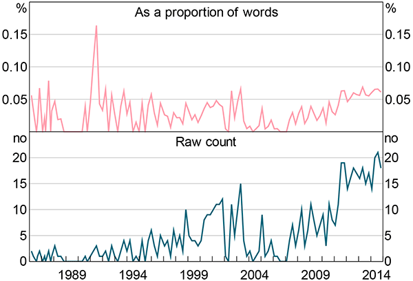
Sources: Author's calculations; RBA
The measure is volatile because ‘uncertain’ is used infrequently. Even in the February 2015 Statement on Monetary Policy (SMP) – the longest to date by words – the word uncertain (or its variants) appears just 27 times in the 80 pages. It is even more infrequent in the earlier part of the sample when the publications most analogous to the SMP were substantially shorter. The measure is also narrow in focus. A more complex measure could assess other likely relevant words such as ‘risk’. I have not done so in order to keep the measure simple, and to follow Baker et al (2015).
Nonetheless, the SMP-based measure is correlated with major events. The measure spikes substantially during the early 1990s recession. It also increases in early to mid 2000, following the bursting of the tech bubble and around the introduction of the goods and services tax.
Jurado, Ludvigson and Ng (2015) create an alternative measure of uncertainty based on the common volatility of forecast misses in a large number of economic series.[32] Unlike other measures reviewed in this paper, their measure of uncertainty captures whether the economy has become more or less forecastable, not more or less volatile. Jurado et al argue that this notion of uncertainty is a better proxy because predictability, not dispersion, matters for economic decision-making. Jurado et al find that their measure differs substantially from other commonly used measures of uncertainty – uncertainty episodes are much less frequent, but more persistent, than other measures imply.
Other measures that have been used in the literature include consumer survey measures of uncertainty (Leduc and Liu 2012) and measures that are based on the dispersion of unit record data, such as: responses to business and consumer surveys (Bachman, Elstner and Sims 2013; Balta et al 2013); and firms' productivity or sales growth (Bachman and Bayer 2013; Bloom et al 2013).
Appendix B: Data Availability for Measures of Uncertainty
| Earliest available data | Frequency | |
|---|---|---|
| Finance-based measures | ||
| Option-implied volatility | January 1995 | Daily(a) |
| Realised All Ordinaries volatility | January 1980 | Daily(a) |
| Analyst earnings forecast uncertainty (ASX 200) | November 2000 | Monthly |
| Analyst earnings forecast uncertainty (by sector) | October 2002 | Monthly |
| Text-based measures | ||
| Proportion of uncertainty-related articles in: | ||
| The Australian | August 1996 | Monthly |
| The AFR | September 1987 | Monthly |
| The Age | August 1991 | Monthly |
| SMH | September 1986 | Monthly |
| SMP-based measure | March 1986 | Quarterly |
| Forecaster disagreement | ||
| RBA survey of market economists – CPI | September 1993 | Quarterly |
| RBA survey of market economists – GDP | December 2008 | Quarterly |
| Consensus Economics – CPI | November 1990 | Monthly |
| Consensus Economics – GDP | November 1990 | Monthly |
| Market economists' cash rate forecasts | April 2009 | Weekly(a) |
| Economic uncertainty index | September 1986 | Monthly |
|
Note: (a) Monthly averages are used in this paper Sources: Author's calculations; Consensus Economics; Factiva; MSCI; RBA; Thomson Reuters |
||
Appendix C: Constructing the Economic Uncertainty Index
C.1 The Components and Construction of the Index
Figure C1 presents the standardised components of the economic uncertainty index.
-
Stock market volatility is constructed from option-implied volatility for the ASX 200 index. Prior to January 1995, the component is constructed from realised volatility of the All Ordinaries index, measured by the monthly average of the absolute value of the daily percentage change in the All Ordinaries index. I rescale the realised volatility measure so that it has the same mean as the option-implied volatility measure over January 1995 to December 2014.
Splicing the two measures together seems reasonable because the forward- and backward-looking measures of stock market volatility line up well. The correlation coefficient between the two series is 0.85 and peaks in the two measures largely coincide. However, the backward-looking measure is more volatile than the forward-looking measure. Over the period for which data exist for both measures, the coefficient of variation for the backward-looking measure is roughly 30 per cent larger.
- Analyst earnings forecast uncertainty is constructed from the coefficient of variation – the cross-sectional standard deviation divided by the mean – of analyst earnings forecasts for ASX 200 companies.
- The uncertainty-related newspaper articles series is the proportion of articles relating to economic uncertainty in The Australian, the AFR, The Age and the SMH. I construct the aggregate series in Figure C1 by standardising the individual newspaper measures over the period for which data exists for all four newspapers to have mean zero and standard deviation of one and then taking an equally weighted average. I use an equally weighted average because I am agnostic about which papers are most influential. Whether an article is related to uncertainty is mechanically determined by a set of search criteria. Not all papers are available for the full sample.
- GDP forecast dispersion is the range between forecasts for GDP growth for the next calendar year from Consensus Economics.
Each of these components is discussed in Section 2.1.
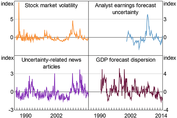
Note: For the period November 2000 to December 2014: all components are standardised to have mean 0 and standard deviation 1
Sources: Author's calculations; Consensus Economics; Factiva; MSCI; Thomson Reuters
In order to construct the index, I demean and standardise all of the components for the period November 2000 to December 2014 to have a standard deviation of one (Figure C1). I then take a weighted average of the components, with 50 per cent weight on the uncertainty-related newspaper articles component, and one-sixth on each of the remaining three components. These weights mirror Baker et al (2015). I then rescale the index so that it has a mean of 100 points and a standard deviation of 30 points for the period November 2000 to December 2014. These choices are arbitrary, and are designed to roughly match the mean and standard deviation of the US economic policy uncertainty index from Baker et al (2015).
C.2 The Three Indices That Make Up the Economic Uncertainty Index
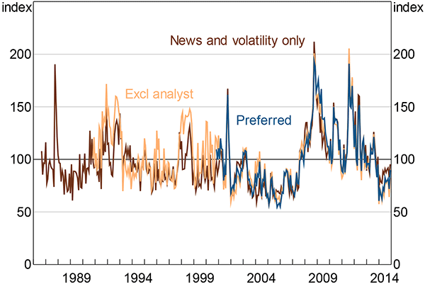
Because the analyst earnings forecast uncertainty series is not available prior to November 2000 and the GDP forecast dispersion series is not available prior to November 1990, I use alternative indices that exclude these components for earlier periods. Each alternative index is scaled to have mean 100 points and standard deviation 30 points for the period November 2000 to December 2014.
For the period November 1990 to November 2000 I use an index that excludes analyst earnings forecast uncertainty (‘excl analyst’). This index is constructed in the same way as the preferred specification index, but with 25 per cent weights on the stock market volatility and GDP forecast dispersion components. For the period September 1986 to October 1990 I use an index that combines the uncertainty-related newspaper articles component and the stock market volatility component with weights of two-thirds and one-third respectively (‘news and volatility only’).
To construct the full-history index in Figure 5, I simply swap to the index containing more data sources as soon as it is available.
The three indices on which the overall index is based are strongly correlated (Table C1). Furthermore, the differences between the three different indices are negligible (Figure C2). The three indices are similar enough that the benefit of having the longer time series outweighs the small differences in comparability between the earlier and later specifications of the index.
| Preferred specification | Excl analyst specification | News and volatility only specification | |
|---|---|---|---|
| Preferred specification | 1 | ||
| Excl analyst specification | 0.98 | 1 | |
| News and volatility only specification | 0.95 | 0.94 | 1 |
|
Notes: Correlations are over the period November 2000 to December 2014, for which data exist for all three indices; all correlations are significant at the 1 per cent level Sources: Author's calculations; Consensus Economics; Factiva; MSCI; Thomson Reuters |
|||
Note: See note to Figure 5
Sources: Author's calculations; Consensus Economics; Factiva; MSCI; Thomson Reuters
C.3 Different Weights
The index is robust to different weights on the components. Figure C3 compares my preferred specification to an equally weighted index and an index where the weights are determined by principal component analysis (PCA).[33] I restrict to the period after November 2000 – the period for which data exist for all four of the components of the preferred specification index. The similarity between differently weighted specifications is unsurprising given the relatively high degree of co-movement among measures of uncertainty (Section 2.1.4).
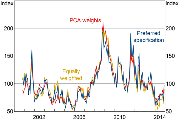
Note: See note to Figure 5
Sources: Author's calculations; Consensus Economics; Factiva; MSCI; Thomson Reuters
Appendix D: Additional Stylised Facts
D.1 Federal Budgets
The story is less clear for federal budgets than for federal elections (Figure D1). The budget month is associated with slightly higher levels of uncertainty, but the months before appear to have lower. Again, because I am not controlling for any other factors, these results simply reflect the average of the index in the relevant month; many other factors are likely at play.[34]
Sources: Author's calculations; Consensus Economics; Factiva; MSCI; Thomson Reuters
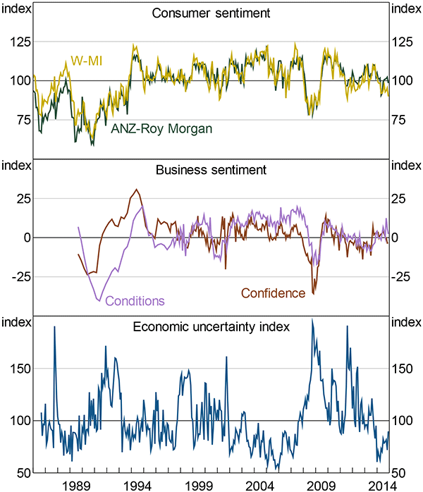
D.2 Sentiment and Uncertainty
One argument against the value of the economic uncertainty index is that measures of sentiment already capture the information contained in the index. However, economic uncertainty is conceptually not the same as sentiment. Business and consumer sentiment indices are about the expected level of future outcomes, while uncertainty is about the dispersion or variance of potential outcomes.
But there is a theoretical reason to expect a small link between the two concepts. Theory predicts that consumption and investment should fall when uncertainty is high. Consumers and businesses should lower their expectations in response.
Notwithstanding the conceptual distinction between the two, the measures of sentiment also likely capture some elements of uncertainty and the economic uncertainty index likely captures some elements of sentiment.
There appears to be some evidence of this ‘contamination’ between the two measures: measures of sentiment decrease when uncertainty increases (Figure D2). For business sentiment, the economic uncertainty index has correlation coefficients of −0.53 and −0.63 with the NAB conditions and confidence indices respectively. For consumer sentiment, the correlation coefficients are −0.32 and −0.25 for the Westpac-Melbourne Institute (W-MI) and ANZ-Roy Morgan indices respectively. All are statistically significant at the 1 per cent level.
Note: The business sentiment measures are from the NAB surveys
Sources: ANZ-Roy Morgan; Author's calculations; Consensus Economics; Factiva; MSCI; NAB; Thomson Reuters; Westpac and Melbourne Institute
Given these correlations, sentiment can explain a large proportion – about 40 per cent – of the variation in the economic uncertainty index (Figure D3).[35] While some of the remaining variation is noise, some of it reflects uncertainty-only shocks – that is, changes in the dispersion of possible outcomes without changes to the expected level of outcomes. The clearest example is the July 2011 US debt ceiling stand-off: sentiment was little changed while the economic uncertainty index reached a near-historic peak. Figure D3 also shows that uncertainty lingered after the Lehman Brothers bankruptcy, even though sentiment recovered.
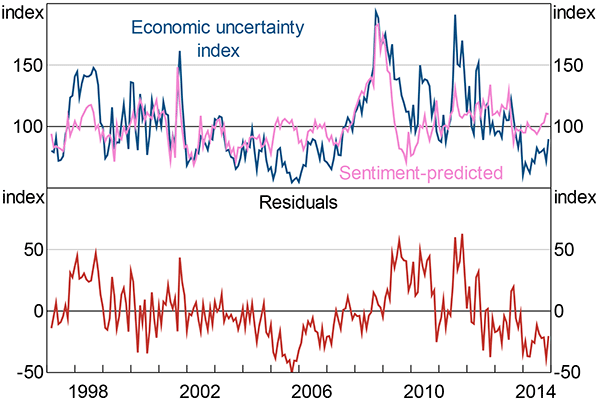
Notes: See note to Figure 5; ‘sentiment-predicted’ is the predicted value of the economic uncertainty index from a regression of the economic uncertainty index on NAB business confidence for the period ahead
Sources: Author's calculations; Consensus Economics; Factiva; MSCI; NAB; Thomson Reuters
Appendix E: Extra VAR Results
E.1 Monthly VAR Robustness
The monthly VAR results are reasonably robust to ordering uncertainty second-last ahead of sentiment and to alternative lag selections (Figure E1). With both two and three lags, there is a somewhat anomalous spike in employment in the two months immediately following the uncertainty shock, but growth is depressed thereafter – consistent with the preferred one lag specification used in Section 4.1.
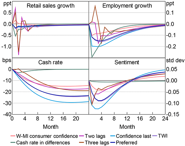
Notes: Retail sales growth and employment growth are annualised; all lines in the cash rate panel show changes in the level of the cash rate, except the ‘cash rate in differences’ series, which shows the change in the cash rate
The results are also robust to using the W-MI measure of consumer sentiment instead of the ANZ-Roy Morgan measure. I also tried including the nominal trade-weighted index, or the US dollar-Australian dollar exchange rate; these made little difference. The results are also robust to using the unemployment rate rather than employment growth.
E.2 Alternative Ordering: Monthly
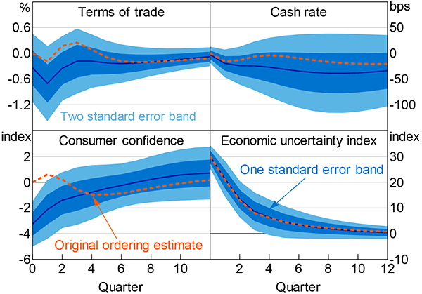
As discussed in Section 4, I use a conservative identification strategy for the main results of the paper: I order the economic uncertainty index last. This means that the only variation that remains in the uncertainty shocks is that which cannot be explained by other variables in the VAR. The estimates presented in Figures 11 and 13 thus represent a kind of lower bound on the effect of uncertainty.
In this section, I flip that identification assumption and order the economic uncertainty index first in the monthly VAR. This restriction assumes that uncertainty contemporaneously affects all other variables, but itself responds only with a lag. Much of the empirical literature uses this ordering.
Unsurprisingly, this alternative identification assumption increases the estimated effects of uncertainty for the monthly VAR. Reassuringly, the differences between these estimates and the main results presented in the paper are small (Figure E2). The close similarity of the responses suggests that little is lost in taking the more conservative identification strategy I use in the text. With either choice of assumptions the broad story that uncertainty matters in Australia does not change.
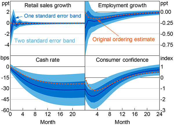
Notes: See notes to Figure 11; the ‘original ordering estimate’ series show the impulse responses from Figure 11
E.3 Other Quarterly Responses
The quarterly responses are reasonably similar to those in the monthly VAR (Figure E3). Consumer confidence has a similar shape, although the response is about half as large in the quarterly VAR and displays an initial peak, similar to investment. The response is much less precisely estimated than in Figure 11 because it is at quarterly frequency. Similarly, the decrease in the cash rate is a little smaller than in the monthly VAR – about one-fifth of a percentage point at peak – although it displays somewhat odd dynamics initially. The terms of trade barely respond to uncertainty shocks. At peak, the change is about one-quarter of a per cent (about a tenth of a standard deviation). Moreover, the response bounces either side of zero.
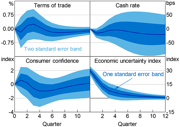
Notes: Consumer confidence (ANZ-Roy Morgan), cash rate and the economic uncertainty index are all quarterly averages; estimation covers June quarter 1987 to December quarter 2014
E.4 Alternative Ordering: Quarterly
As with the monthly VAR, ordering uncertainty first somewhat increases the size of the responses, but does not materially alter the story about how uncertainty affects the Australian economy (Figure E4). The differences in estimated responses are reasonably small between the original ordering and the alternative ordering, although the surprisingly initial increases seen in Figure 13 all but disappear. Naturally, the differences are largest in the first few quarters, where the short-run restrictions of the Cholesky ordering are most binding. After about four quarters the differences between the two sets of estimates are negligible. Again, the similarity of these responses supports the view that taking the more conservative approach in the text carries little cost.
The same is true for the responses of the other variables not shown in Figures 13 and E4. Ordering the economic uncertainty index first in the VAR increases the magnitude of the effects, particularly initially (Figure E5). However, with the possible exception of the cash rate, the differences are neither large nor economically interesting.
Notes: See notes to Figure 13; the ‘original ordering estimate’ series show the impulse responses from Figure 13
Notes: See notes to Figure E3; the ‘original ordering estimate’ series show the impulse responses from Figure E3
E.5 Quarterly VAR Robustness
The quarterly responses are robust to alternative lag specifications, orderings and measures of sentiment (Figure E6). They are also robust to including the nominal TWI, or excluding the terms of trade. There is little variation across the responses, although some measures of sentiment exacerbate the first-quarter spikes.
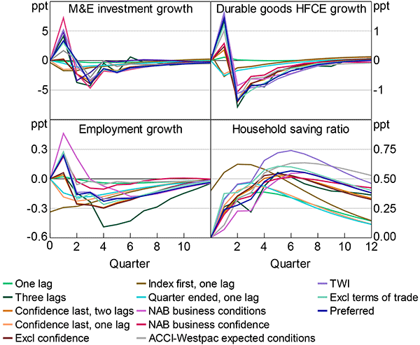
Notes: See notes to Figure 13; the ‘quarter ended, one lag’ series uses the in-month reading for the final month of the quarter; all series use ANZ-Roy Morgan consumer confidence as the measure of sentiment, except the ACCI-Westpac expected conditions, NAB business confidence and NAB business conditions series, which use those measures
The only exception is the ‘one lag’ specification. This specification eliminates the responses of investment, consumption and employment growth (and flips the sign of the response of durable goods HFCE growth). However, the response of the saving ratio is little changed.
This occurs because, with only one lag, the coefficients on uncertainty in the reduced form equations for investment, consumption and employment growth are very close to zero. As a result, uncertainty has little to no direct effect on these variables in this specification. With uncertainty ordered last, sentiment barely responds to an uncertainty shock because the coefficient is also very near zero. However, with uncertainty ordered ahead of sentiment, the uncertainty shock induces a modest-sized contemporaneous fall in sentiment. This fall in sentiment is sufficient to reduce investment, consumption and employment growth. With longer lag structures, uncertainty has a direct effect. This explains why the one-lag uncertainty-last specification produces little to no response, while all the other specifications do – including those with uncertainty ordered last, but longer lag structures.
References
Alexopoulos M and J Cohen (2009), ‘Uncertain Times, Uncertain Measures’, University of Toronto Department of Economics Working Paper 352.
Bachmann R and C Bayer (2011), ‘Uncertainty Business Cycles – Really?’, NBER Working Paper No 16862.
Bachmann R and C Bayer (2013), ‘“Wait-and-See” Business Cycles?’, Journal of Monetary Economics, 60(6), pp 704–719.
Bachmann R, S Elstner and ER Sims (2013), ‘Uncertainty and Economic Activity: Evidence from Business Survey Data’, American Economic Journal: Macroeconomics, 5(2), pp 217–249.
Baker SR and N Bloom (2013), ‘Does Uncertainty Reduce Growth? Using Disasters as Natural Experiments’, NBER Working Paper No 19475.
Baker SR, N Bloom and SJ Davis (2015), ‘Measuring Economic Policy Uncertainty’, NBER Working Paper No 21633.
Balta N, I Valdés Fernández and E Ruscher (2013), ‘Assessing the Impact of Uncertainty on Consumption and Investment’, European Commission Quarterly Report on the Euro Area, 12(2), pp 7–16.
Basu S and B Bundick (2012), ‘Uncertainty Shocks in a Model of Effective Demand’, Federal Reserve Bank of Boston Research Department Working Paper No 12–15.
Bekaert G, M Hoerova and M Lo Duca (2013), ‘Risk, Uncertainty and Monetary Policy’, Journal of Monetary Economics, 60(7), pp 771–788.
Berkelmans L (2005), ‘Credit and Monetary Policy: An Australian SVAR’, RBA Research Discussion Paper No 2005-06.
Bernanke BS (1983), ‘Irreversibility, Uncertainty and Cyclical Investment’, The Quarterly Journal of Economics, 98(1), pp 85–106.
Bloom N (2009), ‘The Impact of Uncertainty Shocks’, Econometrica, 77(3), pp 623–685.
Bloom N (2013), ‘The Macroeconomics of Time-Varying Uncertainty’, IMF Lecture Presentation, Washington DC, 18 January. Available at <http://pages.stern.nyu.edu/~dbackus/BFZ/Literature/Bloom_slides_Jan_13.pdf>.
Bloom N (2014), ‘Fluctuations in Uncertainty’, The Journal of Economic Perspectives, 28(2), pp 153–176.
Bloom N, M Floetotto, N Jaimovich, I Saporta-Eksten and SJ Terry (2013), ‘Really Uncertain Business Cycles’, Centre for Economic Performance CEP Discussion Paper No 1195.
Burns AF and WC Mitchell (1946), Measuring Business Cycles, Studies in Business Cycles, No 2, National Bureau of Economic Research, New York.
Caggiano C, E Castelnuovo and N Groshenny (2014), ‘Uncertainty Shocks and Unemployment Dynamics in U.S. Recessions’, Journal of Monetary Economics, 67, pp 78–92.
Cagliarini A and A Heath (2000), ‘Monetary Policy-Making in the Presence of Knightian Uncertainty’, RBA Research Discussion Paper No 2000-10.
Carriero A, H Mumtaz, K Theodoridis and A Theophilopoulou (2015), ‘The Impact of Uncertainty Shocks under Measurement Error: A Proxy SVAR Approach’, Journal of Money, Credit and Banking, 47(6), pp 1223–1238.
Carroll CD (1997), ‘Buffer-Stock Saving and the Life Cycle/Permanent Income Hypothesis’, The Quarterly Journal of Economics, 112(1), pp 1–55.
Cochrane JH (2011), ‘Presidential Address: Discount Rates’, The Journal of Finance, 66(4), pp 1047–1108.
Davies K (2015), ‘An Economic Policy Uncertainty Index for Australia’, Barclays Australia and New Zealand Economics Weekly, 12 February, pp 2–5.
Dixit AK and RS Pindyck (1994), Investment Under Uncertainty, Princeton University Press, Princeton.
Dungey M and A Pagan (2009), ‘Extending a SVAR Model of the Australian Economy’, Economic Record, 85(268), pp 1–20.
Elias S and C Evans (2014), ‘Cycles in Non-Mining Business Investment’, RBA Bulletin, December, pp 1–6.
FOMC (Federal Open Market Committee) (2009), ‘Minutes of the Federal Open Market Committee December 15–16, 2009’.
Hamilton JD (1989), ‘A New Approach to the Economic Analysis of Nonstationary Time Series and the Business Cycle’, Econometrica, 57(2), pp 357–384.
Jurado K, SC Ludvigson and S Ng (2015), ‘Measuring Uncertainty’, The American Economic Review, 105(3), pp 1177–1216.
Kent C (2014), ‘The Business Cycle in Australia’, Address to the Australian Business Economists, Sydney, 13 November.
Kimball MS (1990), ‘Precautionary Saving in the Small and in the Large’, Econometrica, 58(1), pp 53–73.
Knight FH (1921), Risk, Uncertainty and Profit, Houghton Mifflin Company, Boston.
Lawson J and D Rees (2008), ‘A Sectoral Model of the Australian Economy’, RBA Research Discussion Paper No 2008-01.
Leduc S and Z Liu (2012), ‘Uncertainty, Unemployment, and Inflation’, FRBSF Economic Letter No 2012-28.
Leduc S and Z Liu (2015), ‘Uncertainty Shocks are Aggregate Demand Shocks’, Federal Reserve Bank of San Francisco Working Paper No 2012-10, rev May.
Morley J and J Piger (2012), ‘The Asymmetric Business Cycle’, The Review of Economics and Statistics, 94(1), pp 208–221.
Rich R, J Song and J Tracy (2012), ‘The Measurement and Behavior of Uncertainty: Evidence from the ECB Survey of Professional Forecasters’, Federal Reserve Bank of New York Staff Reports No 588.
Rossi B and T Sekhposyan (2015), ‘Macroeconomic Uncertainty Indices Based on Nowcast and Forecast Error Distributions’, The American Economic Review, 105(5), pp 650–655.
Shiller RJ (1981), ‘Do Stock Prices Move Too Much to be Justified by Subsequent Changes in Dividends’, The American Economic Review, 71(3), pp 421–436.
Tran TL (2014), ‘Uncertainty and Investment: Evidence from Australian Firm Panel Data’, Economic Record, 90(Supplement s1), pp 87–101.
Acknowledgements
I thank Adam Cagliarini, Efrem Castelnuovo, José Dorich, Christian Gillitzer, Bruce Preston, Ewan Rankin, Penelope Smith and John Simon for advice, comments and suggestions. I also thank Stephen Cupper, Virginia Macdonald, Sue Morris and Sean Wang for their assistance collecting data. The views expressed in this paper are mine and do not necessarily reflect the views of the Reserve Bank of Australia. Any errors are my own.
Footnotes
Bloom (2009) presents a model of real options effects in the context of firm hiring and investment choices with adjustment costs. Other earlier contributions to the real options literature include Bernanke (1983) and Dixit and Pindyck (1994). [1]
Appendix B contains a list of the measures reviewed in this section and the time periods for which they are available. Although most of the data in this section are available daily, I use data up to December 2014. [2]
I am extremely grateful to Stephen Cupper and Sue Morris for their assistance in collecting the data used in this section. [3]
Alexopoulos and Cohen (2009) also construct a newspaper-based measure of uncertainty for the United States. [4]
Although there are plausible feedback mechanisms. [5]
I first standardise the individual newspaper measures to have mean zero and standard deviation of one over the period for which data exists for all four newspapers. Articles that are syndicated across more than one of the newspapers will be double counted under this methodology. [6]
I use the monthly average of the absolute value of daily percentage changes because it is most strongly correlated with the option-implied measure over the period for which data exists for both measures (correlation of 0.85). This is in slight contrast to Bloom (2009) and Caggiano et al (2014), who use the within-month standard deviation of daily percentage changes. However, there is little difference between the two series. I use the former measure because it helps mitigate the effect of Black Monday in 1987. The within-month standard deviation measure has a correlation of 0.84 with the option-implied volatility series, very slightly less than the series I choose for realised volatility. [7]
The forward-looking measure of Australian stock market volatility is similar to the closely watched VIX in the United States. [8]
The sample of institutions in the two surveys is similar, so the correlation between dispersion in the two surveys for the same forecast variable is perhaps less surprising. [9]
These data are only available for a relatively short period of time – since April 2009. [10]
History was very unkind to that forecast. [11]
I use GDP rather than CPI forecast dispersion in the economic uncertainty index because it is likely that there is a structural change in CPI forecast dispersion due to the RBA adopting inflation targeting. [12]
The full history is September 1986 to December 2014. [13]
As of an October 2015 revision, Baker et al focus on the uncertainty-related news articles component because it is comparable across countries. The original version of the index that I discuss is still presented as the headline monthly index for the United States on their website, policyuncertainty.com; this index is also available through a number of commercial data providers. [14]
For example, Burns and Mitchell (1946), Hamilton (1989) and Morley and Piger (2012) among many others. [15]
Based on a Shapiro-Wilk test. Additionally, the distribution differs from a normal distribution on both skewness and kurtosis at the 1 per cent level, based on a modified D'Agostino K-squared test. [16]
I also tried a specification that attempted to control for foreign-based uncertainty by using the residuals from the regression of the Australian index on the US index (see the bottom panel of Figure 7). This did not materially alter the results. [17]
In part because there are only 10 elections in the sample, the confidence interval around these estimated effects is large. [18]
The risk premia channel also suggests that uncertainty should reduce investment by raising the cost of capital for firms. I do not address the risk premia channel because I do not have the data necessary to disentangle it from the real options channel. [19]
I use consumer confidence because it has a longer monthly time series than business confidence. In Appendix E.1 I show that the results are robust to using other measures of consumer and business sentiment. [20]
The Akaike Information Criteria (AIC) recommends three lags; the Schwarz Bayesian Information Criteria (BIC) recommends one. [21]
In particular, the retail sales measure is about two-thirds non-durable consumption. This weight is higher than the national accounts measure of goods consumption. In Section 4.2 I use a measure of durable consumption from the quarterly national accounts, which is a much better proxy for discretionary consumption. [22]
The VAR in Figure 12 is otherwise identical to the monthly VAR from Figure 11. [23]
The Australian economic uncertainty index increases about 10 points following a US uncertainty shock. This is broadly consistent with the findings in Section 3.2. [24]
AIC recommends two lags; BIC recommends one. [25]
Using other measures of investment, such as the RBA's estimate of non-mining private business investment (Elias and Evans 2014) or total private business investment, roughly halves the reduction in investment growth, although these are somewhat less volatile series. Other responses are essentially unchanged. [26]
As with M&E investment growth, the initial peak in the quarter following the shock is surprising in light of the sharp and more persistent reversal. [27]
Bloom (2013, 2014) provide comprehensive summaries of the empirical literature. [28]
Baker and Bloom (2013) also use an aggregate-level VAR framework, but incorporate cross-country data and use natural disasters to identify uncertainty shocks. They find much larger effects than I find, but this divergence might reflect differences between Australia and the 60 countries included in Baker and Bloom's dataset, or that the uncertainty shocks they identify – i.e. those related to natural disasters – are different to those that I identify. [29]
Davies (2015) constructs a similar measure for Australia. [30]
I use this normalisation because the publications have increased in length. [31]
Rossi and Sekhposyan (2015) take a similar approach. [32]
The weights for the PCA weights index are: 0.3 on the newspaper-based component; 0.31 on the analyst earnings forecast uncertainty component; 0.34 on the stock market volatility component; and 0.04 on the GDP forecast dispersion component (weights do not sum due to rounding). [33]
As with federal elections (Section 3.5), I tried a specification that attempted to control for foreign-based uncertainty. This did not significantly alter the results. [34]
I use the NAB business confidence series for period-ahead index because it is the best predictor of the variation in the uncertainty index. This might be because both uncertainty and confidence are forward looking. [35]