RDP 2015-07: A Multi-sector Model of the Australian Economy 5. The Model in Action: Scenario Analysis

Having discussed the technical aspects of the model in detail, in the remainder of this paper we put the model to work. The previous section described the model's dynamics using impulse response analysis. This consisted of imposing an innovation to one of the model's structural shocks for a single period and examining the responses of the model's variables to this innovation.

While impulse response analysis is a useful tool for exploring the mechanisms at work in a model, it is rarely informative for policy purposes. Policymakers are typically interested in how the economy will respond after conditioning on an entire path of one or more variables. In this section we use the model to construct this type of scenario.

5.1 Resource Prices and the Exchange Rate

An example of the type of question that the model can address is, ‘How might the economy respond if resource prices were to fall by 10 per cent and remain at that lower level for three years?’. In the previous section we showed that such a development will typically be accompanied by a depreciation of the nominal exchange rate. However, exchange rates are affected by many idiosyncratic factors and there will be instances in which the exchange rate does not respond to a change in resource prices immediately. To account for this possibility, we might put together two variants of this scenario – one in which the exchange rate responds endogenously and one in which the exchange rate is held constant.

Assembling a scenario like the one described above involves a degree of judgement. For example, consider the construction of a constant exchange rate path. Many of the model's shocks affect the exchange rate. One could achieve a constant exchange rate path by applying a sequence of monetary policy shocks, a sequence of consumption preference shocks, a sequence of risk premium shocks or through combinations of those (or other) shocks. The choice matters because the results of the scenario will vary depending on which combination of shocks one uses. In practice, for scenarios like this, we try to use the shocks that are closely related to the variables of interest. For example, in a scenario in which we constrain the path of resource prices and the exchange rate it seems sensible to apply a sequence of resource price and risk premium shocks.^[15]

Another relevant consideration is whether agents anticipate the path of resource prices and the exchange rate. Most of the model's shocks have only transitory effects on real variables and relative prices in economy. So, following a shock that lowers resource prices by 10 per cent, agents will expect resource prices to revert back to their original level gradually. This expectation is inconsistent with the assumption in the scenario that resource prices remain 10 per cent below their initial level for a number of years. In some scenarios, accounting for expectations can have meaningful consequences for model predictions. For example, the response of mining firms to lower resource prices is likely to depend upon whether firms expect resource prices to recover in the future or to remain low for a long period of time.

Our baseline model features only unanticipated shocks. In this set-up, the only way to achieve a prolonged path of lower resource prices in a scenario is to apply a new unanticipated shock each quarter to keep resource prices at their desired level. However, it is straightforward to alter the model's shock structure to allow agents to anticipate the future path of resource prices. To do this, we modify Equation (38) as follows:

where for any j ≥ 1

A positive innovation to increases foreign currency resource prices j periods in the future. One can then use the methods documented in Del Negro, Giannoni and Patterson (2013) to calculate the sequence of shocks required to generate an anticipated path for a given endogenous variable.

5.1.1 Unanticipated shocks and alternative exchange rate scenarios

The first set of results, presented in Figure 8, shows the evolution of key macroeconomic variables for lower resource price scenarios with, and without, an endogenous exchange rate response. We construct these scenarios using a sequence of unanticipated shocks. In the next section we will discuss what happens when we allow agents to anticipate the path of resource prices correctly.

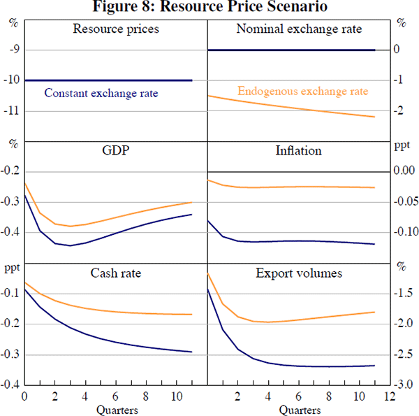
If allowed to respond endogenously, the nominal exchange rate initially depreciates by around 1.5 per cent. If resource prices remain low, it depreciates further in subsequent quarters, reaching around 2.5 per cent below its initial level after three years. A fall in resource prices is contractionary for the economy. However, an exchange rate depreciation reduces the extent of the contraction. When the exchange rate depreciates, the level of output is around 0.1 per cent higher (relative to baseline) than it is in the scenario in which the exchange rate does not depreciate. This largely reflects a different profile for export volumes, which are 0.5 per cent lower after one year if the exchange rate does not depreciate than they are if the exchange rate does depreciate.

The effect of lower resource prices on inflation is estimated to be small. However, inflation falls by more without an exchange rate depreciation because the deflationary effects on non-tradeable inflation are no longer offset by an increase in tradeable inflation. As a consequence, the cash rate also falls by more when the exchange rate does not depreciate, although not by enough to fully offset the additional decrease in output and inflation.

5.1.2 Anticipated versus unanticipated resource price paths

Figure 9 compares the evolution of some key macroeconomic variables for the lower resource price scenario when agents in the model realise that resource prices will be lower for 12 quarters against a scenario in which agents do not anticipate the persistence of the resource price decline. To focus attention on the importance of resource price anticipation, we only show scenarios in which the exchange rate responds endogenously.

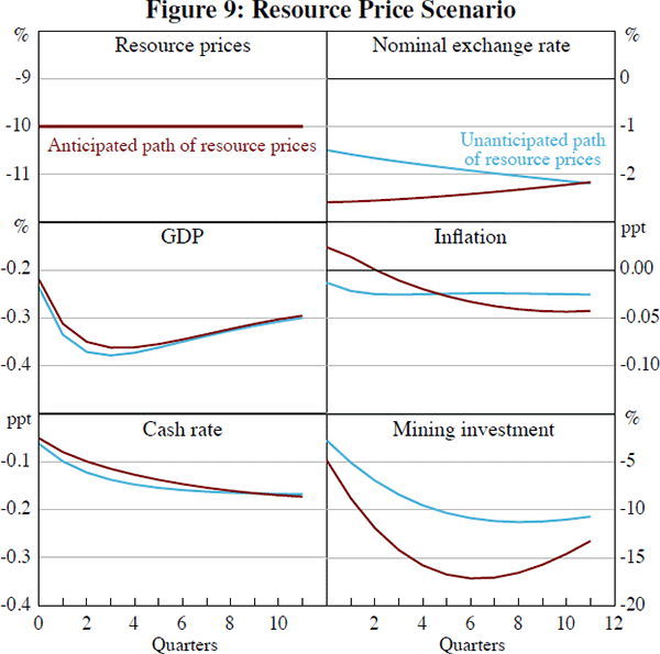
As one might expect, the nominal exchange rate initially depreciates by more when agents correctly anticipate the persistence of the decline in resource prices than it does when agents expect a timely recovery in prices. As a result, inflation also increases by slightly more in the anticipated scenario and the cash rate does not decline by as much.

An important difference between the two scenarios is the behaviour of mining firms. Mining investment falls by almost twice as much when agents realise the decline in resource prices will persist than it does when the decline is expected to be temporary. Despite this, the level of GDP is marginally higher in this scenario. This reflects the additional depreciation of the exchange rate, which ensures that increased exports, and the substitution of domestic consumption and investment from imported to domestic goods, more than offsets reduced expenditure by mining firms.

Footnote

In most instances, if the number of structural shocks equals the number of endogenous variables whose paths one wishes to specify then there is a unique mapping between the sequence of shocks and the desired paths of the endogenous variables. [15]