RDP 2015-04: The Sticky Information Phillips Curve: Evidence for Australia 3. Forecasts
April 2015 – ISSN 1448-5109 (Online)
- Download the Paper 738KB
3.1 Availability and Construction
Estimation of the SIPC requires knowledge of the expected path of inflation and the output gap for each vintage of expectations. Since the early 1990s, Consensus Economics has compiled inflation and GDP growth forecasts based on a survey of professional forecasters.[4] The SIPC requires estimates of changes in the output gap rather than GDP growth but, if we assume that variation in GDP growth is much larger than variation in potential output at short horizons, GDP growth forecasts will provide a suitable proxy.
Official RBA forecasts for CPI inflation, underlying inflation and GDP growth provide an alternative source of expectations data. The RBA has published forecasts of inflation and GDP growth for some period of time, but the full detailed history of forecasts were not made public until 2012. This means that firms could not have used these detailed forecasts to make pricing decisions over the entire sample period. But if similar forecasts were available to firms in real time, the RBA forecasts may provide a reliable guide to expectations. The differences between RBA and Consensus forecasts of CPI inflation and GDP growth have been relatively minor (see Tulip and Wallace (2012)).
Unfortunately, availability of Consensus and RBA forecasts before the low-inflation period is limited. This is a significant weakness, because changes in inflation regimes are a key source of identification for the sticky-information model. Furthermore, the Consensus and RBA forecast horizons are sometimes as short as one year, necessitating truncation of the SIPC at four lags. By constructing econometric forecasts, we can proxy real-time inflation and output gap growth expectations before the low-inflation period, and for longer forecast horizons.
Following Stock and Watson (2003), the econometric forecasts are based on an average of bi-variate h-step-ahead projections. Each regression includes a candidate variable that is believed to have forecasting ability for inflation or growth in the output gap, plus lags of the dependent variable. Averaging across each set of bi-variate forecasts produces the central forecasts for inflation and the change in the output gap. The use of combination forecasts guards against structural change and over-fitting in short samples. Stock and Watson (2004) provide evidence that forecast combination methods provide good out-of-sample forecast performance relative to an autoregressive model. Kahn and Zhu (2006) and Coibion (2010) use a similar forecasting procedure in testing the empirical performance of the SIPC for the United States.
Formally, to forecast variable yt at horizon h, the regression

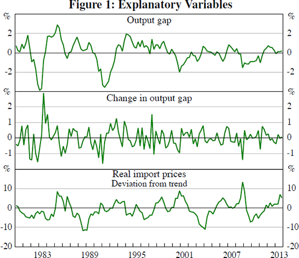
is run for each forecast series yt+h, candidate predictor zt, and forecast horizon h. Each regression includes zt, and up to a maximum of four lags of yt and zt, with lag lengths selected using the Akaike information criterion (AIC). The forecast variables are CPI inflation, underlying inflation and the change in the output gap. Rather than forecasting the output gap and then differencing the forecasts, the change in the output gap is forecast directly. The pseudo real-time output gap xt is estimated from final-vintage GDP data, using a one-sided Hodrick-Prescott (HP) filter.[5] Stock and Watson (1999) report that the one-sided HP-filter produces plausible estimates of the trend component of GDP, without using out-of-sample information. A smoothing parameter of q = 1,600 is used, as is standard for quarterly frequency GDP data. The same one-sided HP-filter is used to detrend real import prices. Figure 1 plots the estimated output gap and import price series.
For forecast horizons between one quarter and two years, the first set of quarterly growth forecasts is generated for 1980:Q1, using a ten-year in-sample period to estimate each variant of Equation (8). The estimation period is then moved forward one quarter at a time to 2013:Q4, generating a full set of forecasts for each horizon. The estimation window for Equation (8) is kept at a fixed ten-year length, allowing for structural change in the parameters of each forecasting regression. The use of out-of-sample rather than in-sample forecasts is critical for evaluation of the SIPC. Ideally, out-of-sample forecasts would be constructed using only real-time data. CPI inflation data are not revised and revisions to underlying inflation data occur only as a result of changes in estimated seasonal factors, but for other series data availability requires the use of final vintage data. Table 1 reports the set of variables zt used to forecast CPI inflation, underlying inflation and the change in the output gap.[6] The selection of these explanatory variables has been guided by Stock and Watson (2003) and Kahn and Zhu (2006). Although few of the variables have a stable forecast relationship over the full sample period, each is likely to contain useful information for forecasting in at least some sub-samples.
| CPI inflation | Underlying inflation | Change in output gap | |
|---|---|---|---|
| Activity | |||
| GDP – quarterly percentage change | ✓ | ✓ | ✓ |
| Output gap | ✓ | ✓ | |
| Capacity utilisation – ACCI-Westpac net balance | ✓ | ||
| Unemployment rate – quarterly change | ✓ | ✓ | ✓ |
| Prices | |||
| Underlying inflation | ✓ | ✓ | |
| Import prices – quarterly percentage change | ✓ | ✓ | ✓ |
| Oil price (AUD) – quarterly percentage change | ✓ | ✓ | ✓ |
| Terms of trade – quarterly percentage change | ✓ | ✓ | ✓ |
| Financial market | |||
| Real trade-weighted index – quarterly percentage change | ✓ | ||
| Share price index – quarterly percentage change | ✓ | ✓ | ✓ |
| Bank bill interest rate – 90-day | ✓ | ✓ | ✓ |
| Yield curve slope – 10-year–90-day | ✓ | ✓ | ✓ |
3.2 Forecast Performance
Table 2 reports the historical performance of each forecast type relative to an autoregressive benchmark. Each number in the table represents the root mean squared error (RMSE) of the forecast relative to the RMSE of an autoregressive forecast; numbers less than unity indicate improved forecast accuracy relative to an autoregressive forecast. Bootstrapped 95 per cent confidence intervals for the econometric forecasts are reported in square brackets.
| Sample period | Forecast horizon | |||||
|---|---|---|---|---|---|---|
| 1-quarter | 2-quarter | 4-quarter | 6-quarter | 8-quarter | ||
| CPI inflation | ||||||
| Consensus | 1995–2013 | 0.65 | 0.72 | 0.80 | ||
| RBA | 1995–2011 | 0.63 | 0.81 | 0.84 | ||
| Econometric | 1995–2013 | 1.02 | 1.05 | 1.05 | 1.04 | 1.05 |
| [0.98, 1.06] | [1.00, 1.09] | [0.99, 1.11] | [0.98, 1.10] | [0.98, 1.12] | ||
| 1980–2013 | 1.00 | 0.98 | 0.93 | 1.01 | 0.96 | |
| [0.97, 1.04] | [0.95, 1.02] | [0.88, 0.97] | [0.96, 1.06] | [0.90, 1.02] | ||
| Underlying inflation | ||||||
| RBA | 1995–2011 | 1.11 | 0.97 | 1.06 | ||
| Econometric | 1995–2013 | 1.00 | 0.96 | 1.03 | 1.04 | 0.98 |
| [0.94, 1.06] | [0.90, 1.03] | [0.95, 1.11] | [0.96, 1.12] | [0.90, 1.06] | ||
| 1980–2013 | 0.93 | 0.94 | 0.85 | 0.96 | 0.98 | |
| [0.88, 0.98] | [0.88, 0.99] | [0.78, 0.90] | [0.89, 1.02] | [0.91, 1.04] | ||
| GDP growth | ||||||
| Consensus | 1995–2013 | 0.99 | 1.01 | 1.09 | ||
| RBA | 1995–2011 | 1.04 | 0.97 | 1.05 | ||
| Econometric | 1995–2013 | 0.98 | 0.98 | 1.04 | 1.03 | 1.03 |
| [0.93, 1.03] | [0.93, 1.03] | [0.99, 1.09] | [0.99, 1.07] | [0.98, 1.07] | ||
| 1980–2013 | 0.97 | 0.97 | 1.04 | 1.00 | 1.02 | |
| [0.93, 1.01] | [0.93, 1.01] | [1.00, 1.07] | [0.97, 1.04] | [0.98, 1.05] | ||
| Note: Where forecast series have been estimated, a 95 per cent bootstrap confidence interval is reported in brackets | ||||||
The Consensus and RBA forecasts substantially outperform the autoregressive CPI inflation forecasts, particularly at a short horizon. At longer horizons, a sizeable portion of the improved forecast performance is due to anticipation of the introduction of the GST in 1999/2000. The CPI inflation series used to estimate the econometric forecasts has been adjusted to remove the effects of tax changes. The econometric forecasts are statistically indistinguishable from the autoregressive benchmark over the low-inflation period, but outperform the autoregressive benchmark at longer horizons over the 1980–2013 sample period. This reflects the fact that inflation has become harder to forecast since the adoption of inflation targeting (see Stock and Watson (2007) for US evidence, and Heath, Roberts and Bulman (2004) for Australian evidence). The results are similar for the underlying inflation forecasts: improved forecast performance relative to the autoregressive benchmark is mostly evident only over the 1980–2013 period. For the GDP growth forecasts, there is little evidence of improved performance relative to the autoregressive benchmark. Where comparable, and except for CPI inflation, the autoregressive forecasts perform similarly well to the official RBA forecasts. Overall, the results presented in Table 2 indicate that the econometric forecasts provide a plausible set of expectations for estimation of the SIPC.
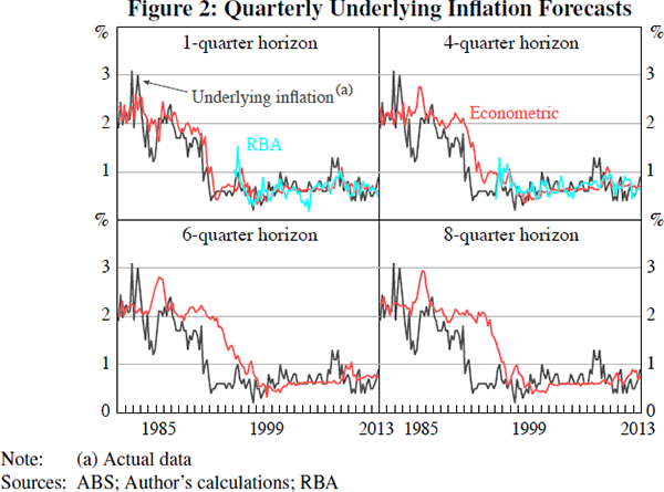
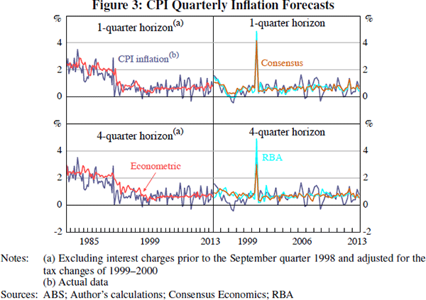
Figure 2 shows the time series of RBA and econometric underlying inflation forecasts, at several horizons. The short-horizon econometric forecasts track measured underlying inflation relatively closely. But the long-horizon econometric forecasts did not predict the early 1990s disinflation. The long-horizon forecasts perform substantially worse than the short-horizon forecasts in the early 1990s because they place a relatively low weight on recent inflation outcomes, and a relatively high weight on real-time estimates of the series mean. The relatively high variability of CPI inflation makes the poor performance of long-horizon forecasts during the disinflation less evident (see Figure 3).
Footnotes
Quarterly inflation and GDP growth forecasts can be inferred from the reported year-ended changes. [4]
The one-sided HP-filter models potential output as an unobserved component, assuming innovations to potential output are uncorrelated with the output gap. [5]
The underlying inflation measure used is: trimmed mean inflation excluding interest charges and tax changes after 1982, non-seasonally adjusted trimmed mean inflation excluding interest charges and tax changes from 1976–1982, Treasury's underlying inflation from 1971–1976, and CPI inflation before 1971. Import prices have been adjusted to include tariff changes. [6]