RDP 2014-03: Household Saving in Australia Appendix A: A Simple Model of Age, Cohort and Time Effects

This model follows the approach of Deaton and Paxson (1994) and Chamon and Prasad (2010), and provides a simple way to disentangle age and birth cohort effects to find their ‘pure’ effect on saving.^[14]

With no shocks to income and a constant real interest rate, the life-cycle hypothesis suggests household consumption can be expressed as:

Here C_ab;h denotes consumption for household h where the household head is aged a and belongs to birth cohort b, f(a) describes how consumption varies with age, W_b denotes the average lifetime resources of households from birth cohort b, and is a (multiplicative) household-specific idiosyncratic shock.

Taking logs and averaging consumption over households in the same age (a) and birth cohort (b) gives

where the age effect – f(a) – is assumed to depend on age but not birth cohort, while lifetime resources – W_b – are assumed to depend on birth cohort but not age. We then use dummy variables to decompose the age, birth cohort and time (i.e. unexplained) components of consumption

Where D^a, D^b and D^t correspond to age, birth cohort and time dummy variables, and α_c, β_c and γ_c correspond to the coefficients capturing age, birth cohort and time effects on consumption.

Since a household's birth cohort is simply a function of the survey year and their age, we need to place some restrictions on the coefficients in this model to enable identification. Following Chamon and Prasad (2010), the birth cohort effects are constrained to sum to zero and be orthogonal to a linear trend:^[15]

Household income (Y) can be modelled in a similar way as

Where α_y, β_y and γ_y correspond to the coefficients capturing age, birth cohort and time effects on income. Similar constraints apply: Σ_iβ_y(i) = 0 and Σ_i(β_y(i)×i) = 0.

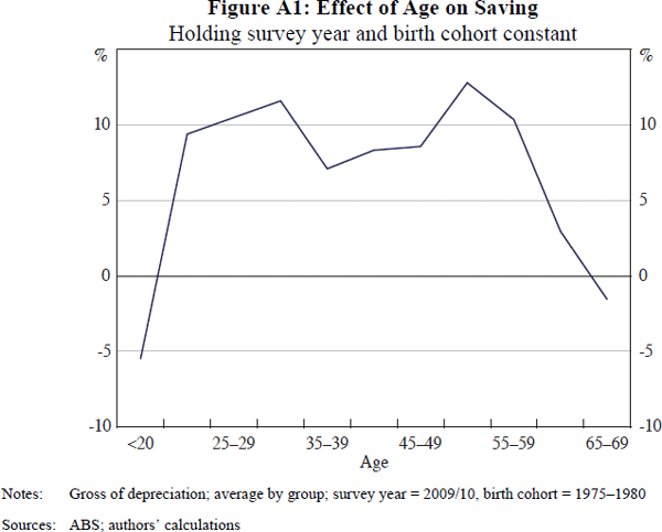
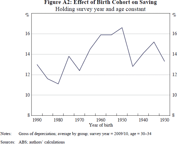
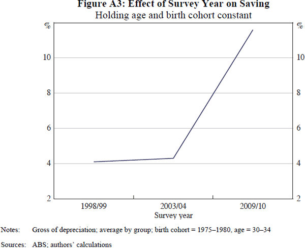
Combining the results of the income and consumption models gives the effect that age, birth cohort and time have on household saving, where household saving ratios are calculated as the difference between the fitted values of the dependent income and consumption variables. Figures A1 to A3 show the estimated effect of age, birth cohort and time respectively, assuming the other effects are held constant. Our reference household for this analysis is a household head aged 30 to 34 surveyed in 2009/10. Note that the level of saving shown in the figures depends on the reference household chosen, but the profile of saving does not, so one should focus on how saving changes for different age, birth cohort or time groups, rather than the level of saving per se.

Focusing on the age effect, Figure A1 shows how the average household's saving ratio varies with age, holding the survey year and birth cohort constant. The distribution of the age effect partially exhibits the concave relationship predicted by the standard life-cycle model; saving is low early and late in life, and high during a household's working years. One anomaly stands out from the standard life-cycle prediction, however: the dip around middle-age (30 to 50 years), when households reduce their saving before building it back up when they enter the preretirement age group.^[16]

A possible explanation for this that accords with a slightly amended life-cycle model is simply that costs increase around middle age. Younger households have relatively few living costs and so are able to save for a down-payment on a house, while middle-aged households have children and must pay mortgage interest. The behaviour is also consistent with a myopic model of household behaviour. For example, Thaler and Shefrin (1981) argue that hyperbolic discounting can explain why younger households tend not to save enough for retirement, while Carroll and Samwick (1997) argue that younger households place more weight on saving for large purchases and emergencies to smooth near-term consumption rather than saving for longer-term (retirement) consumption.

Figure A2 shows how the average household saving ratio varies with birth cohort, holding the survey year and age of the household head constant; the effects are less clear than those for age, although they suggest that the baby boomer cohort (born between 1946 and 1964) saves more than other birth cohorts throughout their lives.

Time effects in this model represent all determinants of saving not relating to age or birth cohort. Between the 1998/99 and 2003/04 Surveys, the time effect on saving is found to be negligible; on the other hand, the time effect between the 2003/04 and 2009/10 Surveys is large and positive (Figure A3).

Footnotes

In this exercise we use the 1988/89, 1993/94, 1998/99, 2003/04 and 2009/10 HES, because a longer time period is needed to determine birth cohort effects precisely. While there were some major methodological changes to pre-1998/99 surveys which make it difficult to compare surveys across time, we assume that the cohort and age effects on consumption and income remain comparable. [14]

As argued in Chamon and Prasad, constraining the time effects would force the decomposition to attribute rising consumption and income to age and/or birth cohort effects, rather than an economy-wide rise in productive capacity. Likewise, restraining the age effects would prevent us from examining the life-cycle hypothesis, which makes predictions about how consumption and income should vary with age. [15]

As noted in Section 2.1, the saving of self-funded retirees, and so the older age groups, is likely to be overstated. [16]