RDP 2013-05: Liquidity Shocks and the US Housing Credit Crisis of 2007–2008 Appendix B: Identifying the Separate Effects of Liquidity and Lending Standards Shocks

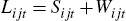
I now modify the model to allow for changes in bank lending standards. I maintain all the assumptions on the demand side of the credit market, but make two slight changes to the supply side. First, identification now requires an assumption that each bank loan to a particular region is ‘locally financed’. For example, if there is a negative funding shock to the Californian subsidiary of Bank of America then that subsidiary cannot obtain replacement finance through an internal transfer from the New York subsidiary. In other words, I assume that it is prohibitively costly for different lending units within a financial institution to cross-subsidise each other's lending. This assumption implies that the flow of funds constraint becomes:

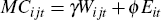
Second, I assume that the bank must exert some costly ‘screening effort’ (E_it) to originate each loan. The effort exerted in screening borrowers can be loosely thought of as the bank's lending standards; a bank that exerts more effort has stricter lending standards. I assume that the cost of screening is given by a convex function . Under this set of assumptions, the marginal cost of lending for the bank is a function of the volume of external finance and the level of screening effort:

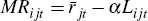
As before, the marginal loan return is given by:

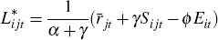
Solving for the first-period equilibrium by equating marginal revenue with marginal cost:

At the end of the first period, the credit market now experiences three shocks. There is the same demand shock as before, but now there are two types of credit supply shocks; there is a liquidity shock and a new shock to screening effort (or ‘lending standards shock’):

1. Credit demand shock:
2. Credit supply (liquidity) shock:
3. Credit supply (lending standards) shock: .

The liquidity shock is similar to before, except that it is now specific to each bank and region (δ_ij) rather than specific to each bank. The new lending standards shock comprises two components: an aggregate shock such as a change in loan screening technology (e.g. the availability of credit scoring), and a bank-specific shock (ψ_i), such as a change in bank risk preferences.

Following the same approach as before, I solve for the second-period equilibrium:

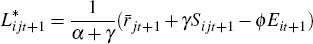
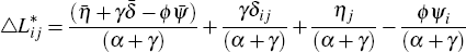
Taking the difference in (equilibrium) lending over time I obtain:

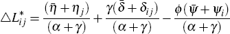
Compared to the basic model, this equation now has an additional term on the right-hand side, which denotes the impact of the lending standards shock. Note that if there is no cost of screening loans (ϕ = 0), then the lending standards shock has no effect on the equilibrium growth rate of lending.

Re-arranging the equation to combine all the aggregate shocks in a single term leads to three separate terms for the bank-region-specific, region-specific and bank-specific shocks:

If the share of loans that are sold (SALESHARE_ij) by each bank in each region is assumed to be a suitable proxy for the liquidity shock (δ_ij) then the following equation can be estimated:

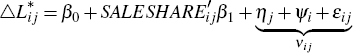
where there is an intercept that captures all the aggregate effects 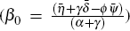, a slope coefficient that captures the relationship of interest, and a composite error term (ν_ij) that includes an unobservable region-specific component (η_j), an unobservable bank-specific component (ψ_i) and a bank-region specific component (ε_ij).

This equation can be estimated by OLS including borrower-specific fixed effects to control for the unobservable credit demand shocks (η_j) and bank-specific fixed effects to control for the unobservable lending standards shocks (ψ_i). An unbiased estimate of the causal effect of the liquidity shock can be obtained by assuming that the share of loans sold by each bank in each region is uncorrelated with the bank-region specific errors (i.e. corr(SALESHARE_ij,ε_ij) = 0).