RDP 2009-10: Global Relative Price Shocks: The Role of Macroeconomic Policies 5. The Shocks
December 2009
A number of shocks to the model are considered and although the focus is on producing multipliers for the effect of each shock on inflation and relative price changes, the shocks are scaled in such as way as to be plausible and to give a crude indication of how much of the observed changes in relative prices from 2002 might be explained within the model.
We first consider a surge in productivity growth in both durable and non-durable manufacturing sectors in developing economies, particularly China. The assumption is that TFP growth in China rises above baseline for a decade before returning to baseline (that is, closing the now smaller gap with the United States at 2 per cent per year). The actual shocks are shown in Table 4; the other economies are scaled to the Chinese shocks as shown. We also set growth in energy, mining and agriculture productivity to zero so that supply shortages emerge gradually over time.
| Productivity growth rate | |
|---|---|
| Energy (all countries) | 0 forever (1.8% below trend) |
| Mining (all countries) | 0 forever (1.8% below trend) |
| Agriculture (all countries) | 0 forever (1.8% below trend) |
| Services (all countries) | Trend |
| Durable manufactures (LATC)(a) | |
| China | 12% above trend for 9 years |
| India | 6% above trend for 9 years |
| Other Asia | 6% above trend for 9 years |
| Latin America | 6% above trend for 9 years |
| Non-durable manufactures (LATC)(a) | |
| China | 12% above trend for 9 years |
| India | 6% above trend for 9 years |
| Other Asia | 6% above trend for 9 years |
| Latin America | 6% above trend for 9 years |
| Risk premia shock | |
| China (all sectors) | −10% forever |
| All other countries and sectors | −5% forever |
| (a) LATC = labour-augmenting technical change | |
The second shock is a fall in global risk, most notable for China, in the form of a reduction in equity risk premium in each sector. This leads to an investment boom in China and some other economies. The scale of the changes to risk premia are also shown in Table 4.
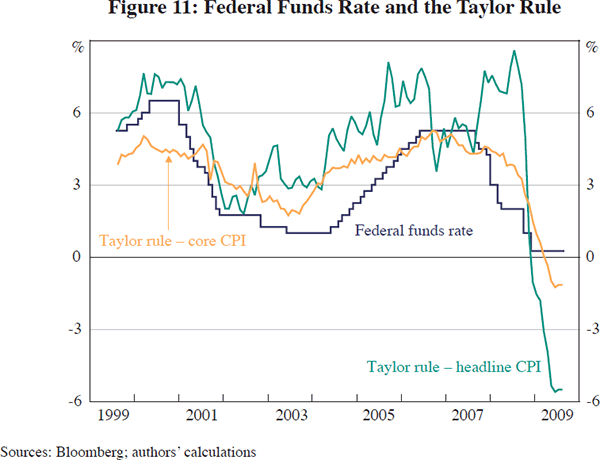
The third shock is to monetary policy over a number of years, with interest rates kept lower than otherwise. The logic for this is as follows. The Taylor rule (also known in the literature in a more general form as the HMT rule) is often used as a guide to measure the level of the short-term nominal interest rate. Between 2001 and 2006, the federal funds rate was below the rate implied by a widely used parameterisation of the Taylor rule by a significant margin (see Taylor 1993, 2009).[4] Using the core PCE measure of inflation, between June 2001 and January 2006, the federal funds rate was below the standard Taylor rule recommendation by an average of around 125 basis points (Figure 11). By this metric, monetary policy was very accommodative during this period. There are a number of ways of trying to engineer a path of interest rates that is below that recommended by some stylised rule. We could use additive shocks to generate a path for interest rates that deviates from the rule. Another way of generating this deviation is to argue that the FRB had assumed a higher growth rate for potential output, thereby lowering their estimation of the output gap leading to lower interest rate settings. Whatever the justification, the key point is that the shocks imply an interest rate path in line with those actually implemented by the FRB from 2001 to 2006.
The size of the shocks we incorporate seem reasonably plausible in light of actual developments over the past seven years or so. The key question then is whether, when combined in the model, they are sufficient to explain the movements of inflation and relative prices over this period. To the extent that the shocks might not be sufficient, other shocks may need to be incorporated into a further analysis, and/or the model may need to be modified in some way.
Footnote
That is, a Taylor rule specified as:  .
The coefficient on the unemployment gap is 1 because there is an implicit
coefficient on the output gap of 0.5 with an ‘Okun's Law’
coefficient of 2. The NAIRU
.
The coefficient on the unemployment gap is 1 because there is an implicit
coefficient on the output gap of 0.5 with an ‘Okun's Law’
coefficient of 2. The NAIRU  is assumed to be 5 per cent and the inflation
target (πT) is 2 per cent.
[4]
is assumed to be 5 per cent and the inflation
target (πT) is 2 per cent.
[4]