RDP 2009-10: Global Relative Price Shocks: The Role of Macroeconomic Policies 6. Results

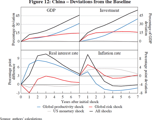
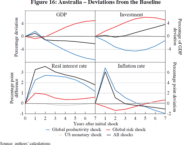
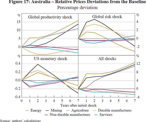
The results of each shock are shown in Figures 12 through 17. These figures display the deviations from the baseline of key variables. Figures 12 and 13 contain results for China, Figures 14 and 15 for the United States, and Figures 16 and 17 for Australia. The figures show the response to each of the three shocks (separately and combined) of: GDP; investment; the real interest rate; and inflation. The responses of prices for each of the six sectors in each economy (relative to the output price index of each economy) are also shown for the combination of the three shocks.

To understand the results it is important to note a key feature of the G-Cubed model. A good produced in a sector within a country is an imperfect substitute for the same good produced in the same sector in another country. Thus, although there are six sectors of production in each country, and each sector within each country has a similar name, in effect there are actually 90 different goods in the model (6 sectors times 15 economies). Every sector has the same production function in each economy, with the same elasticity of substitution between the factors of production. The initial input share coefficients are from recent input-output tables for each economy and differ across sectors and across economies.^[5] Thus mining in China is initially relatively labour intensive whereas mining in Australia is relatively capital intensive.^[6] Since the production technologies to produce investment goods, and goods and services consumed by governments and households have finite elasticities of substitution, there is never complete convergence in the production technologies of the sectors across economies.

6.1 Productivity Shocks

First consider the effect of productivity shocks. The rise in manufacturing productivity in developing economies raises investment in the manufacturing sectors in those economies. The lack of growth in energy, mining and agriculture productivity worldwide tends to retard investment in those sectors. In China, the rise in productivity raises GDP growth and the level of GDP rises further above the baseline each year (Figure 12). Note that the results for GDP in each figure are shown as percentage deviations from the baseline in levels, while the productivity shock is to the growth rate of productivity. Higher productivity growth in manufacturing offsets the low productivity growth in non-manufacturing so that aggregate investment rises and the capital stock grows to the new higher level. Because the shock to the growth rate eventually disappears, the level of GDP and capital will remain permanently higher. Higher expected incomes in China raise consumption. Together with higher investment, aggregate demand temporarily rises above aggregate supply and inflation temporarily rises even though it falls over time. This latter effect follows because the higher growth in China implies that the real exchange rate needs to depreciate (since China has to sell more goods to the rest of the world). Since the nominal exchange rate is fixed, this real depreciation occurs via lower inflation in China (helped about by higher real interest rates).

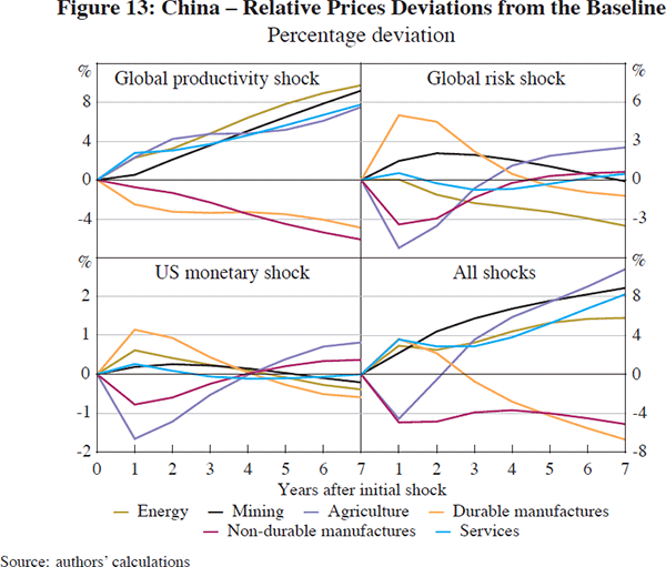
The top-left panel of Figure 13 shows the relative price impacts of the shock to productivity for China. The sectors in which there is strong productivity growth (durable and non-durable manufactures) experience falling input costs and lower prices relative to the economy average. Sectors that are not growing quickly (energy, mining and agriculture) are in greater demand as inputs into manufacturing production but also for higher investment and consumption. Thus the relative prices of these sectors tend to rise as their output becomes increasingly scarce relative to that of the manufacturing sectors. The demand for services also increases as this is a major input into production and consumption. By year 7 the price of energy is 16 per cent higher than the price of non-durable manufactures.

There is an additional important effect on durable versus non-durable goods. A rise in real interest rates tends to reduce the demand for output of the sectors that are producing inputs into capital goods or for goods whose demand depends on the calculation of the present value of a flow of future services. This is particularly an issue for the durable goods sector since it is a large input into producing the investment good that is purchased by all sectors. At the same time, sectors that are relatively capital intensive experience a larger increase in the rental cost of capital and therefore will contract relative to labour-intensive sectors when the real interest rate rises relative to the real wage. In China, the durable goods and energy sectors are capital intensive. Mining is relatively labour intensive in China but relatively capital intensive in the United States and Australia.

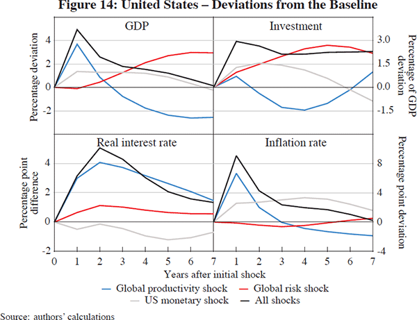
The macroeconomic implications of the rise in developing country productivity for the United States are shown in Figure 14. US GDP rises as a result of the shock in the developing economies, with consumption rising due to higher income from investments in developing economies. However, the GDP increase is short-lived as capital flows from the United States into developing economies in response to higher returns to manufacturing in those economies and due to higher energy and mining prices in the world. The hollowing-out of US manufacturing implies that GDP is 2.5 per cent below baseline by year 7 even though the growth rate of US GDP has returned to its long-run steady state.^[7] The restructuring of US manufacturing also drives the response of aggregate investment (panel 4, Figure 14). While there is additional investment in non-energy sectors, this is outweighed by the decline of manufacturing. The outflow of capital from the United States to developing econommies increases real interest rates in the United States, which further acts to reduce US investment. As for inflation, the initial strength of consumption in the United States, together with higher non-manufacturing prices, is sufficient to initially offset the lower price of imported manufactured goods. However by year 4, the productivity shock is deflationary for the United States.

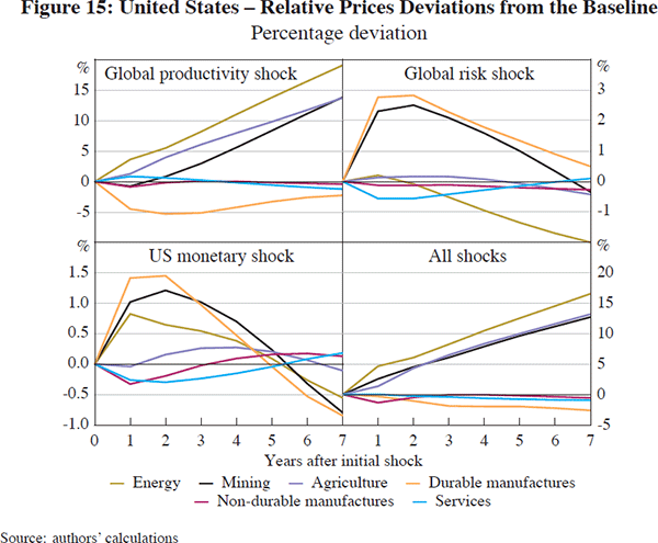
The outcomes for relative prices in the United States are shown in the top left panel of Figure 15. The pattern is very similar to that in China, with the relative price of energy, mining and agriculture rising relative to manufacturing. Despite the manufacturing productivity shock occurring outside the United States, the fall in the relative price of manufactured goods by year 7 in the United States is larger than in China (22 versus 16 per cent respectively).^[8] The one difference between the United States and China, apart from the scale of the response, is that the price of services rises in China whereas it is flat in the United States. This is because there is a larger rise in consumption and, particularly, investment in China, which raises the demand for services by more than in the United States.

The responses in Australia to the productivity shocks are shown in Figure 16 and the top left panel of Figure 17. The results for GDP are similar to the United States in the short run. However, over time the assumption of no productivity growth in the relatively large sectors of the Australia economy – energy, mining and agriculture – weigh heavily on the growth of overall GDP. The increase in the real interest rate also reflects the flow of capital out of Australia into developing economies’ manufacturing sectors, but this effect is smaller than for the United States because there is an inflow of investment into mining for export to the rapidly growing developing economies, which are demanding more raw materials.

6.2 Global Risk Shocks

The reduction in global risk (larger in China than everywhere else) takes the form of a fall in the equity risk premium. The adjustment mechanism in the model occurs through a rise in Tobin's Q for investment in each sector. This causes an investment boom in all countries, especially in China where the shock is largest. As can be seen from the macroeconomic results for China (Figure 12), the United States (Figure 14) and Australia (Figure 16), the adjustment across economies is very similar and as expected. Strong investment raises GDP via short-run demand effects. Over the medium term, GDP rises with the level of potential output, in line with higher capital accumulation. However, there are some subtle differences across countries. In China, monetary policy targets the exchange rate. Whereas real interest rates rise in the United States and Australia – following the initial shock to demand – in China, real interest rates fall initially as otherwise the Chinese currency would tend to appreciate (given the larger decline in the equity risk premium there).

The sectoral story for the risk shock is very different to the results for the productivity shock. As discussed above, the changes in real interest rates relevant to firms and households have very different impacts across sectors depending on how sectoral output is used and on the capital-labour ratio of each sector. The fall in the interest rates faced by households and firms tends to increase the demand for capital-intensive goods, inputs into capital-intensive industries and durable goods. In all economies, the fall in risk premia causes a rise in the demand for durable manufacturing goods and a rise in the relative price of these goods.^[9] Note that mining output rises slightly in China because despite being relatively labour intensive, it is a large input into durable goods production. In both the United States and Australia, where mining is relatively capital intensive, there is a rise in the relative price. Agriculture prices fall sharply in China because agriculture is relatively labour intensive whereas in the United States and Australia, services prices fall by most because they are relatively labour intensive. (Agriculture is more capital intensive in these economies than in China.)

Another interesting insight from the results is that the initial demand change determines the short-run relative price changes in the model. However, over time investment and movements of labour across sectors change the supply side of some sectors. Thus, the medium-term relative price changes reflect a combination of demand and supply effects. So although the price of durable goods increases most in the short run in China, this induces greater investment in durable goods, which expands the supply of these goods and by year 7, the relative price of durables has fallen below the output price index.

6.3 Monetary Policy Shock

The final shock we consider is to monetary policy with the FRB setting policy rates below those implied by a standard Taylor rule. It is useful to start the analysis with the results for the United States shown in Figure 14. The US real interest rate is 50 basis points lower than baseline initially, falling to 1 percentage point below baseline by year 5. This stimulates investment, which raises real GDP above trend for a number of years, but at the same time it pushes up inflation by 2.5 to 3 percentage points. The integral of the difference in real GDP over time is zero because the higher real GDP in the first six years is then followed by GDP below base in subsequent years (not shown).

It is interesting to observe that the change in US monetary policy does change relative prices in the short run (Figure 15). The channel of adjustment is through the impact of real interest rate changes on the demand for durable goods and investment, and depends on the capital intensity of production of different sectors (as discussed above). In year 1, inflation rises by almost 3 percentage points and the price of durable goods relative to non-durable goods rises by 1.7 per cent. As would be expected, this relative price adjustment is largely gone by year 5. The persistence partly reflects the investment changes which propagate a supply response well after the demand response has passed. Thus relative prices overshoot in subsequent years due to the capital accumulation dynamics.

Interestingly, and perhaps not surprisingly, the results for China are very similar to the results for the United States – given that China pegs its currency to the US dollar. Thus the real interest rate falls in China as US monetary policy is relaxed in order to hold the exchange rate fixed. It is difficult to see in Figure 12 because of the scale of the other shocks, but Chinese inflation rises by 3.5 per cent by year 3 as China imports the easier US monetary policy. Chinese real GDP is 1.3 per cent higher by year 2 due to the monetary expansion. Although not as large as the results for the productivity shocks in China, this effect is nonetheless significant. The dispersion of relative price changes in China is also similar to that for the United States and for the same reasons. The one difference again is the mining sector, which is relatively labour intensive in China and therefore does not receive as much stimulus as in the United States where it is relatively capital intensive.

From the results in Figure 16 and 17, it is clear that the floating exchange rate largely insulates the Australian economy from the change in US monetary policy. Real interest rates fall but the effect is small. Nonetheless there are changes in relative prices because of a minor capital intensity effect in Australia, which is due in part to the small change in Australian real interest rates, but more importantly because the United States and China are a large share of the global economy. The dispersion in US relative prices of 1.8 percentage points and in China of 2.7 percentage points is reflected in the dispersion in relative prices in Australia of 0.8 percentage points. The flexible exchange rate only offsets aggregate price relativities but has little influence on the relative price differences across sectors.

6.4 Combining the Shocks

Each of the figures also contains the results of combining all of the shocks in order to get a rough sense of how they offset or reinforce each other. Several interesting insights emerge when compared to the actual experience since 2001. First, while the developing economy productivity shocks are deflationary, this effect is offset by the change in US monetary policy so inflation is largely unchanged in the United States. Hence, from this perspective, US monetary policy appears to have been successful given the announced concern at the time regarding the potential for US deflation after the dot-com bubble burst in 2001.

Second, although the relative prices of energy, mining and agriculture after seven years move in the same direction as that experienced in the world economy over the period 2002 to 2007, the magnitudes are far smaller than the actual experience. The extraordinary magnitudes of the relative price changes between 2005 and 2007 observed in the global economy are not captured by the shocks to fundamentals considered in this modelling exercise. The sharp rise in the relative prices of commodities in excess of the model simulations could be explained by three different causes: speculative activities not built into the analysis in this paper; a set of shocks not considered in this paper; or misspecification of the model (that is, the model may not adequately reflect reality).

Footnotes

We use the GTAP 6 Data Base as detailed in Dimaranan (2006). [5]

The relative intensities can change as relative prices adjust to shocks. So, for example, if the wage-rental ratio increases in China, mining may become more capital intensive there. [6]

While GDP in the United States falls below baseline, the United States receives higher income from investments abroad and faces lower prices for imports and other goods. So even though production in the United States is below baseline, real incomes are higher and US households are better off overall. [7]

Demand for manufactured goods is relatively weaker in the United States, given that Chinese income directly benefits from the higher level of productivity there. [8]

This effect is particularly important for understanding the consequences of the global financial crisis on durable goods production and trade in the context of a large increase in risk premia. See McKibbin and Stoeckel (2009). [9]