RDP 2006-01: Modelling Manufactured Exports: Evidence from Australian States 4. Methodology
April 2006
- Download the Paper 484KB
4.1 Cointegration
Examining the profile of exports and trading partner GDP strongly suggests that these series are non-stationary, so that any regression of exports on trading partner GDP will produce spurious results if these series are not cointegrated. However, cointegration between these series is likely, given that exports are typically assumed to grow in line with trading partner GDP, adjusted for movements in competitiveness.
A range of unit root tests were conducted on the variables of interest to determine their appropriate order of integration. Exports for all states except Tasmania, and trading partner GDP for all states were found to be non-stationary using the Kwiatkowski et al (1992) test (the KPSS test). However, it is unclear whether these series are I(1) or trend stationary; neither the KPSS test of stationarity nor the Perron and Ng (1996) test of non-stationarity can reject their respective hypotheses when a trend is included in the export or trading partner GDP series. With regard to each state's real exchange rate, KPSS tests cannot reject the hypothesis of stationarity for all states except Tasmania. In summary, it is clear that exports are either I(1) or trend-stationary for all states except Tasmania, trading partner GDP is either I(1) or trend-stationary for all states, and real exchange rates are stationary, in general.
Several methods are used to test for cointegration, with the results summarised in Table 4.[7] First, the Engle-Granger (1987) test finds that the residuals from a regression of exports on a constant, the level of the real exchange rate and trading partner GDP are stationary in all states, indicating cointegration. However, this test has been found to have low power, and an alternative test based on the significance of the coefficient on the error-correction term in an error-correction model has been proposed by Kremers, Ericsson and Dolado (1992). Using the modified version of this test suggested by Zivot (1994), cointegration is found for all states, although only at the 10 per cent level for NSW and Victoria. Finally, the Johansen (1991) systems cointegration test was also used; this test finds evidence of cointegration in all states.
| Cointegration test | |||
|---|---|---|---|
| Engle-Granger (ADF statistic) |
Zivot alpha test (t-statistic) |
Johansen (trace statistic) |
|
| Vic | −4.83** | −1.96* | 45.2** |
| NSW | −3.48** | −1.78* | 45.3** |
| SA | −5.35** | −2.32** | 50.5** |
| WA | −3.39** | −3.21** | 49.3** |
| Q1d | −3.69** | −3.33** | 42.5** |
|
Notes: * and ** denote significance at the 10 and 5 per cent levels respectively. The Engle-Granger test is an Augmented Dickey-Fuller test on the residuals of a regression of exports on trading partner GDP and the real exchange rate, with a 5 per cent critical value of 3.29 (Engle and Yoo 1987). The Zivot alpha test is a t-test of the coefficient on the residuals from the above regression when included in an error-correction model of manufactured exports; this test is distributed normally, with 5 per cent critical value of −2.00. The Johansen test is a systems test of the rank of the matrix of cointegrating vectors, and is conducted with a constant included in the cointegrating vector; the 5 per cent critical value for this statistic is 35.2. | |||
In short, it is clear that both exports and trading partner GDP are non-stationary and, on the assumption that they are I(1), exports, trading partner GDP and the real exchange rate are cointegrated for all mainland states. In this case, it seems appropriate to estimate the long-run relationship between these variables, using cointegration techniques. Alternatively, if exports and trading partner GDP are trend-stationary, standard regression techniques are valid and these same cointegration techniques are appropriate. The following section discusses these techniques in further detail.
4.2 Specification
Two alternative specifications are used to estimate the cointegrated equations, the dynamic ordinary least squares (DOLS) and autoregressive distributed lag (ADL) models.[8] Following Stock and Watson (1993), the DOLS model take the following form:
where: xs,t is the volume of manufactured exports in state s; zs,t is a (column) vector of the real exchange rate and trading partner GDP for each state; and θs is a (row) vector of long-run elasticities with respect to the real exchange rate and trading partner GDP (all variables are in natural logs). The Newey-West (1987) covariance matrix is used to account for serial correlation, and leads and lags of the first-differenced regressors are included to remove correlation between the regressors and the error terms. Consistent with Pesaran and Shin (1998), the ADL model is estimated as follows:

where the long-run price and income elasticities are defined as θs = φ/(1−∑pδp). Appropriate lag lengths, p and q, are chosen by minimising the Schwarz information criteria for each state. Standard errors for the long-run elasticities can then be estimated using a Bewley (1979) transformation:

with xt-i-1 instrumenting Δxt-i. Both DOLS and ADL specifications have been found to perform well in a Monte Carlo analysis of small-sample cointegrated equations (see, for example, Stock and Watson 1993 and Panopoulou and Pittis 2004).
4.3 Panel Estimation
For each of these models specifications, two panel methods are used to estimate national elasticities. The first is the mean-group panel, where each state equation is estimated allowing elasticities to vary across states, and a single national elasticity estimate is then calculated as the weighted average of each state's elasticity (where the weights are each state's share of national exports, excluding Tasmania and the territories). To improve the efficiency of the estimates, and allow for the likely correlation of residuals across states, all five state regressions are jointly estimated using the Generalised Methods of Moments estimator, allowing for both auto-and cross-correlation of the residuals. Pesaran and Smith (1995) suggest using this mean-group approach when elasticities are heterogeneous, which may occur here given that factors often thought to influence the elasticity of exports vary across states. Elasticities are likely to vary according to market power, which may depend, among other things, on the share of elaborately transformed goods in total manufactured exports; highly skilled products requiring elaborate transformation tend to have fewer direct competitors and hence less negative price elasticities (Figure 3). Products with a higher import share of production are also likely to have less negative elasticities, given that the price of imports will fall in domestic-currency terms following an appreciation, allowing exporters to maintain world-currency prices while still maintaining margins. On this basis, we would expect Victoria and South Australia to have smaller elasticities (in absolute terms) than other states, given their high share of elaborately transformed products and imported inputs in production, while Queensland and Western Australia are likely to have larger (absolute) elasticities.
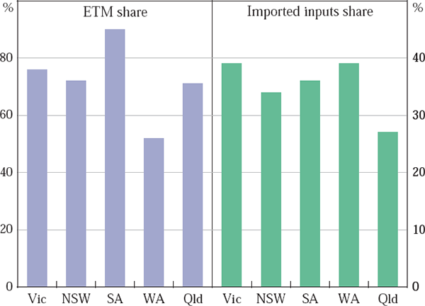
Notes: ETM share is calculated as the share of manufactured exports, using 2-digit SITC data that are elaborately transformed, using 2000–2004 data. The imported inputs share is calculated from 1999/2000 data.
A second approach is to use a fixed-effects panel, which constrains all states' elasticities to be common but allows for differences in intercepts. This specification saves on degrees of freedom and is therefore potentially more efficient than the mean-group method. However, it will produce inconsistent estimates if elasticities are not equal across states (Pesaran and Smith 1995).[9] The DOLS and ADL specifications are used to estimate the fixed-effects model. Following Mark and Sul (2003), only coefficients on the elasticity terms are constrained in this panel, with coefficients on the lags and leads (where present) assumed to vary across states.
Footnotes
Given that Tasmanian exports are stationary, cointegration tests do not apply. Furthermore, it is inappropriate to model (stationary) exports as a function of (non-stationary) trading partner GDP. Given the small size of Tasmania's manufactured exports, and the desire for a consistent modelling approach, its exports are not studied further in this paper. [7]
Johansen's (1991) vector error-correction model is frequently used with cointegrated systems, but it is not used in this paper because its desirable properties in the face of endogeneity are not likely to be relevant for this study, and in small samples it can produce estimates with large variance and non-normal errors. [8]
This is due to two problems; first, a single vector will not cointegrate for all states with heterogenous long-run elasticities, leading to spurious results; and second, if the regressors are serially correlated, this will also cause the residuals to be serially correlated. However, Rebucci (2000) suggests that these concerns may not be important if the time series is sufficiently large. [9]