RDP 2005-06: Credit and Monetary Policy: An Australian SVAR 3. Estimation and Results
September 2005
- Download the Paper 205KB
In the model, inflation is expressed as a quarterly percentage change and the cash rate is expressed in percentage points. All other variables are in logs. The model is estimated for the period that starts with the float of the Australian dollar, in 1983:Q4, and ends in 2003:Q4. This is a similar sample period to that used in most Australian VAR studies. Standard errors for the impulse response functions are calculated using the bootstrap procedure from Kilian (1998).
3.1 Lag Length
Table 1 reports serial correlation tests using different lag lengths of the reduced form VAR. On the basis of these results it is not clear what is the appropriate lag length for the VAR. There is weak evidence of first or fourth order serial correlation for almost all lag lengths. Other Australian studies have tended toward shorter lag lengths; Dungey and Pagan (2000) used three lags and Suzuki (2004) used only two. One exception is Brischetto and Voss (1999), whose model contains six lags. A lag length of three was chosen for this study as this provides reasonable dynamics without shortening the estimation sample too much. Section 3.4 demonstrates that the main results are robust to the lag length chosen.
| Lag | comm | usgdp | gdp | π | cred | i | twi |
|---|---|---|---|---|---|---|---|
| First order serial correlation | |||||||
| 2 | 0.29 | 0.00 | 0.66 | 0.06 | 0.24 | 0.01 | 0.99 |
| 3 | 0.03 | 0.32 | 0.63 | 0.03 | 0.70 | 0.61 | 0.82 |
| 4 | 0.01 | 0.74 | 0.45 | 0.30 | 0.59 | 0.40 | 0.37 |
| 5 | 0.43 | 0.18 | 0.51 | 0.76 | 0.24 | 0.27 | 0.29 |
| 6 | 0.13 | 0.09 | 0.11 | 0.24 | 0.09 | 0.34 | 0.11 |
| 7 | 0.12 | 0.20 | 0.14 | 0.13 | 0.33 | 0.02 | 0.69 |
| 8 | 0.11 | 0.39 | 0.94 | 0.60 | 0.57 | 0.21 | 0.79 |
| 9 | 0.53 | 0.56 | 0.04 | 0.24 | 0.63 | 0.03 | 0.05 |
| Fourth order serial correlation | |||||||
| 2 | 0.15 | 0.01 | 0.04 | 0.01 | 0.03 | 0.08 | 0.02 |
| 3 | 0.01 | 0.39 | 0.02 | 0.12 | 0.06 | 0.50 | 0.00 |
| 4 | 0.04 | 0.35 | 0.13 | 0.24 | 0.39 | 0.69 | 0.00 |
| 5 | 0.79 | 0.32 | 0.65 | 0.05 | 0.10 | 0.60 | 0.03 |
| 6 | 0.26 | 0.20 | 0.14 | 0.16 | 0.24 | 0.08 | 0.29 |
| 7 | 0.09 | 0.49 | 0.07 | 0.25 | 0.24 | 0.02 | 0.65 |
| 8 | 0.38 | 0.49 | 0.92 | 0.33 | 0.52 | 0.67 | 0.94 |
| 9 | 0.61 | 0.62 | 0.25 | 0.04 | 0.08 | 0.01 | 0.00 |
3.2 Impulse Responses and Variance Decomposition
Impulse responses provide a useful summary of the relationships implied by the large number of estimated coefficients in the VAR. The impulse responses can be constructed for shocks to any of the variables in the model. In this paper, only the impulse responses for shocks to the cash rate and credit are presented. VAR studies often highlight the response of the economy to monetary shocks, and so impulse responses to a cash rate shock allow a useful comparison with previous studies and a check on the properties of the model. The impulse responses for shocks to credit, and the cash rate, help to highlight the interaction of credit with the rest of the economy.
Figure 1 shows the impulse responses to a structural cash rate shock that increases the interest rate by 25 basis points.[6] These show the deviation of each variable from its baseline. Given that all variables, other than the (quarterly) rate of inflation and the cash rate, are in log form, multiplication by 100 yields the approximate percentage deviation from baseline. The dashed lines are 90 per cent confidence intervals derived using the technique of Kilian (1998).
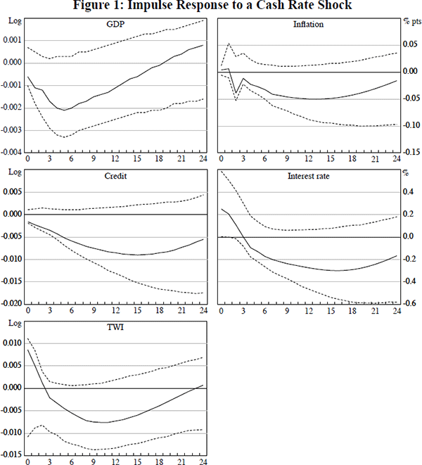
The shock to the cash rate leads to an instantaneous appreciation of the exchange rate of almost 1 per cent. The increase in the cash rate results in a very small contemporaneous fall in credit which in turn leads to a small fall in GDP and a very small pick-up in inflation.
After the initial shock, the cash rate steadily declines until it is roughly back to baseline three quarters after the shock. It continues to decline for three more years – at which time it is around 25 basis points below baseline – in response to the paths of the other variables, notably the declines in inflation and output. It then gradually picks up.
GDP declines steadily in the year after the shock, to be about 0.2 per cent lower after five quarters. Following a volatile estimated response in the first year, inflation steadily declines. The maximal response of inflation is about three years after the shock when the quarterly rate of inflation is 0.05 percentage points lower than baseline. The relatively slow response of inflation to a cash rate shock is a well-established result. The timing of the maximum impact on output and inflation is broadly consistent with previous studies for Australia (Brischetto and Voss 1999; Dungey and Pagan 2000).
Credit responds more slowly to the cash rate shock than does GDP. In fact the timing of its response is more akin to that of inflation. Credit is 0.5 per cent below counterfactual levels after five quarters. It continues to fall until it is almost 1 per cent lower after four years, before it begins to recover. It is interesting to note that while the initial response is small, credit appears to respond immediately to the cash rate shock. In contrast, as noted in Section 1, many studies have found that credit only declines in response to an interest rate rise with a lag. Often these studies have used only bank credit, because they have focused on the credit channel. Nevertheless, the immediate response of credit to monetary policy in this SVAR was found to be robust to using only the component of credit provided by banks.
Following the initial appreciation, the exchange rate depreciates, consistent with uncovered interest rate parity. However, it should be noted that the Killian-bootstrapped 90 per cent confidence intervals for all of the impulse response functions are quite wide, so that none of the results are statistically significant at conventional confidence levels. While the impulse responses are not statistically significant, the point estimates are still economically significant, and numerically and qualitatively plausible.
The effect on GDP reported here is somewhat larger than that reported in other studies, for example Dungey and Pagan (2000) and Brischetto and Voss (1999). However, due to the size of the standard errors, there is scope to reconcile the results. By and large, the results for other variables fall within the range that has been established elsewhere.
An alternative method of interpreting the properties of the model is with a variance decomposition. This reports the proportions of the error of forecasts, generated by the SVAR, that are attributable to shocks to each of the variables in the model. The variance decompositions for four different forecast horizons (one quarter, and one, three and six years) are reported in Table 2. Each column reports, for a different domestic variable, the proportion of the forecast error that is explained by structural shocks to each of the seven explanatory variables, listed on the left-hand side of the table (so, for a given time horizon, the entries in a given column sum to one, subject to small differences for rounding).
| Innovation | Forecast | Proportion of forecast error variance for variable | ||||
|---|---|---|---|---|---|---|
| (quarters) | gdp | π | cred | i | twi | |
| comm | 1 | 0.00 | 0.00 | 0.03 | 0.00 | 0.06 |
| 4 | 0.07 | 0.11 | 0.01 | 0.04 | 0.11 | |
| 12 | 0.10 | 0.22 | 0.04 | 0.03 | 0.24 | |
| 24 | 0.28 | 0.45 | 0.44 | 0.32 | 0.18 | |
| usgdp | 1 | 0.14 | 0.00 | 0.03 | 0.00 | 0.00 |
| 4 | 0.27 | 0.03 | 0.17 | 0.00 | 0.03 | |
| 12 | 0.52 | 0.05 | 0.12 | 0.03 | 0.18 | |
| 24 | 0.61 | 0.10 | 0.05 | 0.13 | 0.28 | |
| gdp | 1 | 0.57 | 0.02 | 0.01 | 0.01 | 0.01 |
| 4 | 0.32 | 0.03 | 0.06 | 0.01 | 0.04 | |
| 12 | 0.14 | 0.10 | 0.15 | 0.08 | 0.17 | |
| 24 | 0.04 | 0.09 | 0.12 | 0.11 | 0.16 | |
| π | 1 | 0.18 | 0.97 | 0.01 | 0.02 | 0.04 |
| 4 | 0.21 | 0.67 | 0.05 | 0.19 | 0.02 | |
| 12 | 0.15 | 0.42 | 0.29 | 0.37 | 0.13 | |
| 24 | 0.05 | 0.26 | 0.24 | 0.27 | 0.17 | |
| cred | 1 | 0.04 | 0.00 | 0.39 | 0.43 | 0.15 |
| 4 | 0.01 | 0.07 | 0.19 | 0.43 | 0.10 | |
| 12 | 0.00 | 0.03 | 0.03 | 0.15 | 0.02 | |
| 24 | 0.00 | 0.01 | 0.01 | 0.03 | 0.01 | |
| i | 1 | 0.04 | 0.00 | 0.34 | 0.34 | 0.27 |
| 4 | 0.08 | 0.06 | 0.24 | 0.20 | 0.15 | |
| 12 | 0.08 | 0.11 | 0.23 | 0.18 | 0.11 | |
| 24 | 0.02 | 0.07 | 0.11 | 0.10 | 0.10 | |
| twi | 1 | 0.02 | 0.00 | 0.20 | 0.20 | 0.46 |
| 4 | 0.05 | 0.03 | 0.28 | 0.14 | 0.55 | |
| 12 | 0.01 | 0.06 | 0.14 | 0.17 | 0.14 | |
| 24 | 0.01 | 0.02 | 0.03 | 0.04 | 0.09 | |
In the short run, shocks to inflation and GDP's own shocks are important for GDP forecast errors. But as the horizon lengthens, the exogenous global variables, US GDP and commodity prices, play a greater role. This is consistent with previous studies, such as Brischetto and Voss (1999), Dungey and Pagan (2000) and Kim and Roubini (2000). For inflation, its own shocks are responsible for almost all of the short-term forecast error. Over longer horizons, shocks to commodity prices are increasingly important. Shocks to the interest rate have been only a small part of GDP and inflation forecast errors. This too is consistent with many other studies. It is also eminently sensible that an arguably stationary variable such as interest rates has little influence on a trending variable such as GDP in the long run.
Over short horizons, the forecast errors for credit are explained by shocks to credit itself, the interest rate and the exchange rate. Not surprisingly, at longer horizons shocks to major macroeconomic variables – output, inflation and commodity prices – play a greater role. This finding is related to a broader pattern observed in these decompositions. Table 2 shows that innovations to the international variables become more important as time passes across the spectrum of domestic variables. This reflects the role that these exogenous factors play in determining the long-run values of the domestic variables in this type of model.
3.3 The Impact of Monetary Policy and Credit Shocks
Standard impulse response functions describe the response of the system to an exogenous shock, say to the interest rate, but with the paths of all variables, including the shocked variable, endogenously determined. It is this endogenous determination that results in the interest rate in Figure 1 declining after the initial shock to be below baseline after one year. So these impulse responses jointly summarise the response of the variables to an initial cash rate shock and the ongoing endogenous response of the cash rate. In many regards, understanding the impact of the systematic component of policy, that is the part that is the endogenous response to observable changes in the economy, is of greater interest (McCallum 1999).
One method to examine this systematic component of policy is to compare the impulse responses when policy responds endogenously to the case in which monetary policy is passive, and so the interest rate remains constant at the initial shocked level. This exercise is of course subject to the Lucas critique given that the behaviour embodied in the equations for the other variables has been estimated when monetary policy has been responsive. Nevertheless, other studies have adopted similar strategies, accepting the problems associated with this exercise.[7] Sims and Zha and Bernanke et al noted that this experiment implies that the public are surprised by the passivity of interest rates and interpret this as random deviations from the underlying model. As a result, the plausibility of this experiment diminishes at longer time horizons.
Figure 2 presents these constrained impulse responses (passive monetary policy), along with the unconstrained impulse responses (endogenous monetary policy) from Figure 1, for a structural interest rate shock that increases the cash rate by 25 basis points.
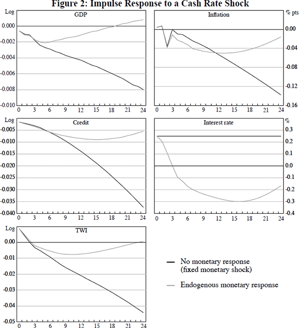
For the first year the constrained and unconstrained impulse responses are almost identical (other than for the interest rate, of course). Thereafter, they begin to deviate. This demonstrates that much of the behaviour of the other variables in the first year is dictated by the initial shock, with the subsequent endogenous response of the interest rate over the first year doing little to unwind these effects. But after the first year the easing in policy from the endogenous response of the cash rate clearly does have an effect, with GDP, inflation, credit and the exchange rate all returning toward baseline. Notably, of all the variables, inflation and credit have the slowest divergence between the constrained and unconstrained impulse responses. This highlights the relatively long lags with which monetary policy affects both inflation and credit.
This technique of comparing the impulse responses when monetary policy is constrained and responds endogenously is also particularly useful for elaborating on the relationship between credit and monetary policy. In particular, it can be used to examine the implications of monetary policy's reaction to a credit shock. Sims and Zha (1998) and Brischetto and Voss (1999) also investigate the consequences of constraining monetary policy in the face of a shock to a non-policy variable. Figure 3 plots the impulse responses for a structural shock of a 1 per cent increase in credit both with passive (constrained), and endogenous (unconstrained), monetary policy. (In this scenario the impulse responses are based on the same size structural shock, rather than the same size reduced form shock as for the cash rate shock in Figures 1 and 2. This allows the impact of the instantaneous response of monetary policy to be considered).
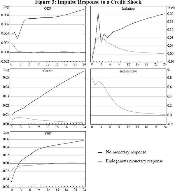
The impulse response for endogenous monetary policy shows that the credit shock leads to a sizeable increase in the interest rate (the constrained interest rate impulse response is zero by definition). It should be noted though, that this does not imply that monetary policy responds directly to credit movements in and of themselves. Rather, the endogenous changes in monetary policy are the response to all of the variables in the system, notably inflation and output.
The endogenous setting of monetary policy is seemingly quite effective at mitigating the impact of credit shocks. The effects of monetary policy in this case are particularly marked for GDP and the exchange rate, with both experiencing substantially smaller deviations from baseline when policy responds. While inflation picks up in response to the credit shock even when the interest rate is increased, the response is more muted as a result of the policy response.
3.4 Robustness
SVARs can be quite sensitive to the assumptions used in their estimation; see for example Stock and Watson (1996, 2001). In particular, changes to the sample length and the number of lags in the VAR can have large effects. The robustness of the estimates to these factors is considered in this section.
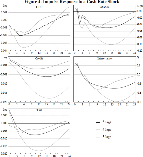
The impulse responses for a structural interest rate shock that increases the cash rate by a 25 basis point reduced form shock to the cash rate for the original specification with three lags, and SVAR models that include four and five lags (but use the same identification restrictions), are shown in Figure 4. The contemporaneous endogenous response of the cash rate differs between these specifications and so a different structural shock must be applied in each case to deliver the 25 basis point reduced form shock.[8] In contrast to the sensitivity of some VAR models to the lag length, Figure 4 demonstrates that the SVAR used in this paper is quite robust to the lag length. In particular, the impulse responses for all variables have broadly the same shape and very similar timing.
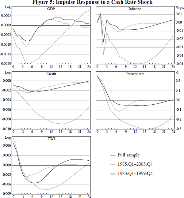
The sample period used to estimate the SVAR covers some major changes in the Australian economy, notably reform in the financial sector and the adoption of inflation targeting. The robustness of the results with respect to the sample period is tested by estimating the model for two truncated samples. The first sub-sample removes the first two years (and so covers 1985:Q4–2003:Q4) while the second removes the last two years (1983:Q4–2001:Q4). Shorter sub-samples are not really practical because of the large number of parameters to estimate. The impulse responses to a monetary shock for the standard SVAR estimated over these sub-samples are shown in Figure 5, along with the impulse response based on the full sample. Each model is subject to a structural interest rate shock that increases the cash rate by 25 basis points.[9] The broad patterns are similar under the three specifications, though the model is more sensitive to the sample period than it was to the lag length. The effects of the interest rate shock on GDP, inflation and credit are not as persistent in the two sub-samples. What is common to the two two-year blocks that are excluded to form the sub-samples is that real credit was accelerating very strongly. Further, the muted response of GDP and inflation to an interest rate shock when estimating from 1985:Q4 appears to be influenced by excluding the sharp rise in the cash rate in 1984–1985, which was followed by declines in GDP and inflation. Nonetheless, the sign and timing of the response is reasonably robust to the sample length, especially in comparison to the sensitivity that other authors, including Brischetto and Voss (1999), have found.
The robustness of the model along other dimensions was also examined, though these are not reported for brevity. When the data are detrended, as in Dungey and Pagan (2000), the effects of a monetary policy shock tend to be more persistent, though the efficacy of monetary policy in dealing with credit shocks is almost identical to the results presented in this paper. Similar conclusions are reached when the first difference of the levels series are used in place of the levels data.
Footnotes
This paper presents impulse responses for reduced form interest rate shocks of 25 basis points, rather than structural shocks of a given magnitude, as often used in VAR studies. This makes comparisons across different specifications straightforward as the initial movement in the interest rate is always the same magnitude. Because of the contemporaneous relationships, the structural shock that results in a 25 basis point reduced form shock is larger – 57 basis points for this specification. The way this is determined is by scaling the structural shock to the interest rate, which is the sixth element of ut, so that the sixth element of the vector εt in Equation (A1) in Appendix A is ‘+0.25’, as determined by the relationship Bεt = ut. [6]
Examples are Sims and Zha (1998), Brischetto and Voss (1999) and Bernanke, Gertler and Watson (1997). However, there is a slight difference between the exercise performed in this section and the exercise performed by Sims and Zha. Sims and Zha assume that the monetary variables still respond to their own lags, so the policy variables are not above (or below, depending on the shock) counterfactual values by a fixed constant. [7]
For the models with 3, 4 and 5 lags the structural shocks are, respectively, 57, 82 and 28 basis points. [8]
Again, the structural shock which results in a 25 basis point reduced form shock differs in each model. In the 1985:Q4–2003:Q4 and 1983:Q4–2001:Q4 samples it is 32 and 42 basis points, respectively; slightly smaller than 57 basis points in the full sample. [9]