RDP 2005-05: Underlying Inflation: Concepts, Measurement and Performance 3. Properties of Underlying Inflation Measures
July 2005
- Download the Paper 192KB
This section examines the features of a range of underlying inflation measures calculated for Australia, assesses any bias with respect to CPI inflation, and considers their performance as indicated by the ‘gap’ test described earlier. The measures considered are: the double-weighted measure;[12] the 30 per cent symmetric trimmed mean and the symmetric weighted median; the optimal Jarque-Bera trimmed mean discussed in the previous section; and two exclusion-based measures published by the Australian Bureau of Statistics (ABS) – the CPI excluding volatile items and market prices excluding volatile items. The trimmed means are calculated in three ways: first, using unadjusted quarterly price changes; second, using seasonally adjusted quarterly price changes; and third, using year-ended price changes. The double-weighted measure is calculated using unadjusted and seasonally adjusted quarterly price change data.
Measures based on the distributions of seasonally adjusted quarterly price changes and annual price changes are considered because the prices of certain items display identifiable seasonality in a yearly cycle.[13] Although in aggregate the Australian CPI is not particularly seasonal (Australian Bureau of Statistics 2004), several items in the distribution of price changes (for example, health, education, utilities and property rates & charges) do display significant seasonality. Seasonal analysis of the disaggregated quarterly price changes can be performed using packages such as the US Census Bureau's X12-ARIMA program.[14] A seasonal analysis of the Australian data revealed that in total, around one-third of the CPI expenditure classes display significant seasonality.[15] Sliding spans analysis was applied to all series with a sufficiently long run of data, and only those series with seasonal factors found to be robust on this basis were accepted as seasonal. Applying X12-ARIMA seasonal factors to the associated CPI components enabled the construction of a new distribution of price changes, from which ‘seasonally adjusted’ measures of core inflation could be calculated.
An alternative method of accounting for seasonality in the disaggregated price data is to calculate underlying inflation rates on the basis of the distribution of four-quarter-ended price changes. Since seasonal items often record large increases only once a year, seasonality observed in the quarterly data often ‘washes out’ of the year-ended calculation. For the aggregate CPI and the exclusion-based measures, the four-quarter-ended price change is the same whether it is calculated directly or from compounding the quarterly movements, because the weighted mean calculation is linear. Likewise, the double-weighted measure presented in this paper will only differ for year-ended inflation data if the weights are recalculated on a four-quarter-ended basis. But the weighted median and trimmed mean can be quite different when calculated on a different basis.
The way in which the Australian CPI is constructed creates practical problems for utilising the four-quarter-ended distribution. Changes to the CPI basket, which occur roughly at five-year intervals, but which have been slightly more frequent in the past ten years, mean that while a continuous time series of quarterly price-change distributions can be obtained, there are gaps in the series of four-quarter-ended distributions. This prevents a four-quarter-ended weighted median, trimmed mean and optimal Jarque-Bera trim from being directly calculated in a transition period. The statistics corresponding to these measures shown in this paper are therefore based on interpolated data.[16]
Table 3 considers the average variability of the different underlying inflation measures. Two alternative sample periods are shown: 1987:Q1 to 2004:Q4 and 1993:Q1 to 2004:Q4. The earlier period is the longest over which data are available for all measures, while the inflation-targeting period, which starts in 1993, is a logical alternative for analysis, given that it corresponds to a period of low and stable inflation. Unsurprisingly, all of the underlying inflation measures shown are less volatile than CPI inflation for both sample periods. The exclusion-based measures, which remove specified items whose prices are deemed particularly volatile in every period, are the most volatile of all the underlying inflation measures. It also bears noting that the volatility-weighted measures themselves do not necessarily display significantly lower volatility than the other measures. This is not surprising, as trimmed means with substantial trims weight the least volatile components more heavily and give a zero weight to the most volatile components. It is also apparent that seasonally adjusting the disaggregated data makes little difference to the variability of a given statistical underlying inflation measure. Finally, the measures based on the distribution of annual price changes are less volatile than year-ended CPI inflation. Differences between the three types of underlying inflation measure become more distinct when the question of bias is considered.
| Indicator | 1987:Q1–2004:Q4 | 1993:Q1–2004:Q4 |
|---|---|---|
| Quarterly | ||
| Consumer Price Index | 0.57 | 0.30 |
| Quarterly measures: not seasonally adjusted | ||
| Weighted median | 0.49 | 0.19 |
| 30 per cent trimmed mean | 0.46 | 0.17 |
| Market prices excluding volatile items | 0.53 | 0.26 |
| CPI excluding volatile items | 0.52 | 0.24 |
| Optimal Jarque-Bera trim | 0.47 | 0.19 |
| Double-weighted measure | 0.48 | 0.21 |
| Quarterly measures: seasonally adjusted | ||
| Weighted median | 0.48 | 0.17 |
| 30 per cent trimmed mean | 0.47 | 0.17 |
| Optimal Jarque-Bera trim | 0.47 | 0.18 |
| Double-weighted measure | 0.46 | 0.20 |
| Year-ended | ||
| Consumer Price Index | 2.09 | 0.67 |
| Measures based on the annual distribution of price changes(b) | ||
| Weighted median | 2.05 | 0.53 |
| 30 per cent trimmed mean | 2.02 | 0.48 |
| Optimal Jarque-Bera trim | 2.02 | 0.53 |
| Notes: (a) All series exclude interest charges and tax effects. (b) Interpolated. |
||
3.1 Average Inflation and Bias
Table 4 shows summary statistics for this selection of measures, calculated on a year-ended basis. Looking first at the unadjusted quarterly measures, it is apparent that the weighted median, trimmed mean and market prices excluding volatile items measures all show an average negative bias of 0.2 percentage points or more with respect to CPI inflation. The optimal Jarque-Bera trimmed mean also displays a (smaller) downward bias. Compared with more standard trimmed means, the optimal Jarque-Bera trim on average excludes a substantially lower percentage of the price change distribution (around 8 per cent) in addition to being – at least in principle – more robust to departures from normality in the original distribution of price changes. The double-weighted measure and the CPI excluding volatile items measure display a lower degree of bias than the other measures. Only in the cases of the trimmed mean and the market prices excluding volatile items is the bias statistically significant.
| Indicator | Average | |
|---|---|---|
| 1987:Q1–2004:Q4 | 1993:Q1–2004:Q4 | |
| Consumer Price Index | 3.62 | 2.48 |
| Quarterly measures: not seasonally adjusted | ||
| Weighted median | 3.40 | 2.26 |
| 30 per cent trimmed mean | 3.37* | 2.25** |
| Market prices excluding volatile items | 3.12* | 2.20** |
| CPI excluding volatile items | 3.38 | 2.42 |
| Optimal Jarque-Bera trim | 3.36 | 2.24 |
| Double-weighted measure | 3.58 | 2.44 |
| Quarterly measures: seasonally adjusted | ||
| Weighted median | 3.51 | 2.36 |
| 30 per cent trimmed mean | 3.57 | 2.44 |
| Optimal Jarque-Bera trim | 3.53 | 2.37 |
| Double-weighted measure | 3.86 | 2.80 |
| Measures based on the annual distribution of price changes(b) | ||
| Weighted median | 3.56 | 2.42 |
| 30 per cent trimmed mean | 3.56 | 2.40 |
| Optimal Jarque-Bera trim | 3.54 | 2.38 |
| Notes: ** and * denote statistically significant bias at the 5 and 10 per
cent levels, respectively. (a) All series exclude interest charges and tax effects. (b) Interpolated. These measures are not tested for bias. |
||
Turning to the seasonally adjusted measures in Table 4, it is apparent that the observed negative bias is negligible for the weighted median, the trimmed mean and the optimal Jarque-Bera trim. The double-weighted measure, indeed, has a positive bias when calculated using seasonally adjusted price changes. None of these biases is statistically significant.[17] It is also apparent from Table 4 that none of the measures based on the distribution of annual price changes is substantially biased. These findings suggest that, in general, seasonally adjusted quarterly measures and measures based on the distribution of annual price changes may be more appropriate than the unadjusted quarterly measures for assessing the underlying inflation rate.
3.2 Explaining the Presence or Absence of Bias
Why is it that underlying inflation measures based on unadjusted quarterly data display a downward bias while those based on seasonally adjusted data or year-ended price changes do not? As far as (unadjusted) quarterly trimmed means are concerned, it is often the case that items displaying large increases once or twice a year are trimmed from the distribution of price changes in the quarters when they record their largest increases, resulting in a lower average inflation rate over the year for trimmed measures than for the published CPI. Seasonally adjusting price changes at the disaggregated level can eliminate biases caused in this way, by smoothing price changes over the course of a year. This reduces the chance that a highly seasonal item will be trimmed from the distribution of price changes, providing that inflation over the year in that item is not significantly greater than overall CPI inflation.[18] As shown in Section 2.2, the pharmaceuticals component is one of the items most frequently removed by the symmetric 30 per cent trimmed mean. But when these prices are seasonally adjusted it is removed far less frequently. The same is true of many other items, including domestic holiday travel & accommodation, education, electricity and property rates & charges, all of which are removed roughly half as frequently when seasonally adjusted.
A similar explanation can be given for the lack of bias observed in measures based on the distribution of year-ended price changes. By smoothing seasonal price spikes over the course of a year, the four-quarter-ended calculation eliminates the effect of regular seasonality in determining which items are trimmed. Several items that display significant seasonality are removed from the annual distribution much less frequently than they are from the quarterly distribution (for example, automotive fuel, pharmaceuticals and domestic holiday travel & accommodation).[19]
While the seasonally adjusted underlying inflation measures and the measures based on the distribution of year-ended price changes do not display significant bias with respect to CPI inflation, a few caveats are worth noting. First, measures based on seasonally adjusted price changes are subject to revision as new inflation data become available. For a number of highly seasonal component series, such as those in the education category, only a short sample of data is available (with as few as 19 observations). Hence, the corresponding seasonal factors may not prove stable in the longer term.[20] Second, any changes in observed seasonal patterns, or the appearance of temporary atypical seasonality in specific items, could potentially affect the signal provided by these measures. The extent to which this is a first- or second-order empirical issue has yet to be established for Australian data.
While there is no strong a priori reason to prefer measures calculated using the quarterly rather than the four-quarter-ended distribution, as discussed previously the fact that three observations are lost in each transition period means that interpolated data must be used. It would also be difficult to derive an informative quarterly series from the annual data using mechanical techniques, although this need not diminish the value of the annual interpolated series as an analytical tool. In the absence of a corresponding quarterly series, this paper does not attempt to use econometric criteria to assess measures based on the distribution of annual price changes. But to the extent that these measures are less biased with respect to CPI inflation than the unadjusted quarterly measures, they still have a useful role to play in the assessment of underlying inflationary trends.
3.3 Econometric Assessment of Underlying Inflation Measures
We first present the results of the ‘gap’ test described in Section 2.3 to determine whether
CPI inflation adjusts towards underlying inflation measures. The results are
displayed in Table 5. For each sample the estimates of
γ11 and γ21 in Equations
(3) and (4) are presented. It is apparent that, for the 1987:Q1–2004:Q4
sample, the coefficient γ11 is statistically significant
for all of the underlying inflation measures considered, irrespective of whether
or not they are based on seasonally adjusted data, suggesting that CPI inflation
tends to move towards each underlying inflation measure. In addition, in all
but two cases it is clear that underlying inflation does not adjust towards
the CPI inflation rate – that is,  is statistically insignificant. The exceptions are the unadjusted and seasonally
adjusted trimmed means, for which
is statistically insignificant. The exceptions are the unadjusted and seasonally
adjusted trimmed means, for which  is significantly less than zero.
| 1987:Q1–2004:Q4 (72 observations) |
1993:Q1–2004:Q4 (48 observations) |
||||
|---|---|---|---|---|---|
 |
 |
 |
|
||
| Quarterly measures: not seasonally adjusted | |||||
| Weighted median | −1.20 (0.00)*** |
−0.08 (0.43) |
−0.85 (0.00)*** |
0.16 (0.27) |
|
| 30 per cent trimmed mean | −1.48 (0.00)*** |
−0.35 (0.01)*** |
−1.32 (0.00)*** |
−0.22 (0.12) |
|
| Market prices excluding volatile items | −1.01 (0.00)*** |
0.15 (0.29) |
−0.85 (0.00)*** |
0.27 (0.04)** |
|
| CPI excluding volatile items | −1.26 (0.00)*** |
−0.15 (0.39) |
−1.12 (0.00)*** |
0.03 (0.85) |
|
| Optimal Jarque-Bera trim | −1.24 (0.00)*** |
−0.10 (0.27) |
−1.10 (0.00)*** |
−0.01 (0.92) |
|
| Double-weighted measure | −1.18 (0.00)*** |
−0.07 (0.47) |
−0.86 (0.00)*** |
0.16 (0.14) |
|
| Quarterly measures: seasonally adjusted | |||||
| Weighted median | −1.28 (0.00)*** |
−0.12 (0.16) |
−0.92 (0.00)*** |
0.08 (0.51) |
|
| 30 per cent trimmed mean | −1.48 (0.00)*** |
−0.30 (0.00)*** |
−1.20 (0.00)*** |
−0.09 (0.44) |
|
| Optimal Jarque-Bera trim | −1.22 (0.00)*** |
−0.05 (0.52) |
−1.00 (0.00)*** |
0.06 (0.61) |
|
| Double-weighted measure | −1.19 (0.00)*** |
−0.09 (0.59) |
−0.90 (0.00)*** |
0.07 (0.20) |
|
| Notes: *** and ** denote significance at the 1 and 5 per cent levels, respectively; p-values are given in parentheses. The estimated coefficients refer to the parameters in Equations (3) and (4). | |||||
At first glance, the results for the 1993:Q1–2004:Q4 sample appear to suggest
that the same proposition holds – i.e., that there is strong evidence
that CPI inflation moves towards the various underlying inflation measures.
These results should be treated with some caution, however, because the implicit
restriction underlying the gap test referred to in Section 2.3, which broadly holds
for the longer sample, does not hold for this shorter sample
period.[21]
To obtain a clearer picture of what is going on in the shorter sample, we estimate
Equation (6) to perform the augmented gap test, as discussed in Section 2.3.
It will be recalled that this equation simply augments the gap regression with
the term  .
In this case,
.
In this case,  refers to the mean of CPI inflation for the
1993:Q1–2004:Q4 sample, which is 0.6 per cent per quarter, or 2½
per cent in annualised terms. Table 6 shows the results of estimating Equation
(6) for the 1993:Q1–2004:Q4 sample.
refers to the mean of CPI inflation for the
1993:Q1–2004:Q4 sample, which is 0.6 per cent per quarter, or 2½
per cent in annualised terms. Table 6 shows the results of estimating Equation
(6) for the 1993:Q1–2004:Q4 sample.
| 1993:Q1–2004:Q4 (48 observations) | |||
|---|---|---|---|
 10 10 |
11 |
12 |
|
| Quarterly measures: not seasonally adjusted | |||
| Weighted median | 0.00 (0.89) |
0.08 (0.78) |
−0.99 (0.00)*** |
| 30 per cent trimmed mean | 0.00 (0.47) |
−0.64 (0.10)* |
−0.56 (0.04)** |
| Market prices excluding volatile items | 0.00 (0.54) |
−0.40 (0.04)** |
−0.70 (0.00)*** |
| CPI excluding volatile items | 0.00 (0.93) |
−0.37 (0.20) |
−0.80 (0.00)*** |
| Optimal Jarque-Bera | 0.00 (0.49) |
−0.57 (0.04)** |
−0.56 (0.02)** |
| Double-weighted measure | 0.00 (0.91) |
−0.28 (0.24) |
−0.72 (0.00)*** |
| Quarterly measures: seasonally adjusted | |||
| Weighted median | 0.00 (0.94) |
−0.17 (0.57) |
−0.82 (0.06)* |
| 30 per cent trimmed mean | 0.00 (0.93) |
−0.50 (0.17) |
−0.62 (0.03)** |
| Optimal Jarque-Bera trim | 0.00 (0.84) |
−0.40 (0.16) |
−0.65 (0.01)** |
| Double-weighted measure | 0.00 (0.62) |
−0.28 (0.24) |
−0.71 (0.01)*** |
| Notes: ***, ** and * denote significance at the 1, 5 and 10 per cent levels, respectively; p-values are given in parentheses. The estimated coefficients refer to the parameters in Equation (6). | |||
It is apparent from Table 6 that in all cases the coefficient ( 12)
on the difference between CPI inflation and
12)
on the difference between CPI inflation and  is significantly less
than zero. This implies that when CPI inflation has departed from its average
of 2½ per cent in annualised terms, it has tended to adjust towards
that average rate in the following quarter. This finding is consistent with
the results of Heath et al (2004) indicating that CPI inflation
is, statistically, explained reasonably well by a constant over this sample
period.
is significantly less
than zero. This implies that when CPI inflation has departed from its average
of 2½ per cent in annualised terms, it has tended to adjust towards
that average rate in the following quarter. This finding is consistent with
the results of Heath et al (2004) indicating that CPI inflation
is, statistically, explained reasonably well by a constant over this sample
period.
The coefficient on the underlying inflation term (11)
is also significantly less than zero in the cases of the unadjusted trimmed
mean, the market prices excluding volatile items measure, and the optimal Jarque-Bera
trim. However, the coefficient is insignificant at ordinary levels of confidence
for the four seasonally adjusted measures. Nonetheless, for a number of cases
in which 11
is statistically insignificant, it appears that this coefficient may still
be economically significant. A good example is the regression involving the
seasonally adjusted trimmed mean, which has an estimated coefficient of 11
= −0.5. This coefficient suggests that when a gap emerges between CPI
inflation and the trimmed mean inflation rate, CPI inflation typically adjusts
half of the way towards the trimmed mean inflation rate in the following quarter.
Broadly similar results hold for the seasonally adjusted optimal Jarque-Bera
trim and several of the unadjusted measures.
This economic interpretation of the coefficient 11
suggests that CPI inflation partially adjusts towards measures of underlying
inflation when a gap opens up between CPI inflation and the underlying inflation
measure in question. The fact that several of the quarterly underlying inflation
measures display this property implies that they can be viewed as providing
useful supplementary information concerning the ‘trend’ in inflation
in the 1993:Q1–2004:Q4 sample period. As noted above, the results from
the longer sample, which contains considerably more variation, suggest that
all of the measures considered satisfy this minimum property. Therefore, it
seems that the analysis of inflationary trends could benefit from the application
of a number of these measures.
In practice, however, it is clear that some measures will be more useful than others for assessing the current trend in inflation. Trimmed means calculated using disaggregated price data that have been seasonally adjusted and measures based on the annual distribution of price changes both tend to be unbiased with respect to CPI inflation. The observed bias in the market prices excluding volatile items measure cannot be remedied in this fashion. In addition, as explained in Section 2, the fact that exclusion-based measures cannot be relied upon to exclude appropriate components from the CPI on a regular basis suggests more generally that they should be used with caution.
Even when bias has been corrected, however, different measures give different signals from time to time. Figure 1 displays the time-series properties of the seasonally adjusted trimmed mean, the trimmed mean based on the annual distribution of price changes, and CPI inflation.
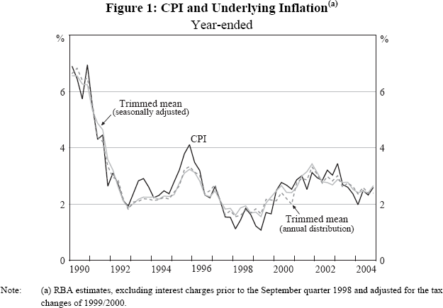
It is apparent that all three series tend to co-move. However, at times the two underlying inflation measures give somewhat different signals regarding the trend in inflation (for example, in early 2000 and late 2001 the two measures move briefly in opposite directions). The same is true of other underlying inflation measures considered in this paper. As individual measures may be inaccurate guides to the underlying trend in a given quarter, there is thus justification for an approach to analysing underlying inflation that relies more on a ‘suite’ of underlying inflation measures than on any single measure.[22]
Footnotes
The weights used in the construction of the double-weighted measure are CPI effective expenditure weights multiplied by reciprocals of the variances of disaggregated price changes (calculated for the entire sample). This is the standard ad hoc construction. See the Appendix for further details on this measure. [12]
Seasonal adjustment has been employed by several authors to improve empirical estimates of core inflation. See Bryan and Cecchetti (1999) and Aucremanne (2000), for applications to Japanese and Belgian data, respectively. [13]
See the Census Bureau's website for more information: <http://www.census.gov/srd/www/x12a/>. [14]
The number of CPI expenditure classes varies between 89 and 107 depending on which period is being considered. [15]
The interpolation method used is as follows. For each break period there are three quarters for which four-quarter-ended price changes are not available. Denote as quarter t the last quarter for which four-quarter-ended data for the ‘old’ series are available (that is, the quarter prior to the break). The first quarter of the break period is then denoted t+1, the second t+2 and the third t+3. The annual rate to quarter t+1 is calculated by compounding the (aggregate) three-quarter-ended statistical measure for t with the quarter-on-quarter statistical measure for t+1. The second quarter is interpolated by compounding the two-quarter-ended statistical measure for t with the two-quarter-ended statistical measure for t+2. The third quarter is interpolated by compounding the quarter-on-quarter statistical measure for t with the three-quarter-ended statistical measure for t+3. As the interpolated figures may be biased downwards due to differences between higher- and lower-frequency distributions, a bias adjustment is made to each figure, estimated by averaging the bias for the calculation of the corresponding period (for example, the March quarter) over the previous four equivalent periods (that is, the previous four March quarters). [16]
Nonetheless, the bias for the double-weighted measure is sufficiently large to warrant caution interpreting this measure in practice. The fact that the measure based on unadjusted data exhibits negligible bias suggests that seasonal adjustment is probably not necessary for this measure. [17]
A similar point is made by Aucremanne (2000), in reference to Belgian CPI data. [18]
On a more abstract level, it is worth noting that measures based on distributions of price changes calculated for very high frequencies are in general likely to yield downwardly biased estimates of underlying inflation. As an extreme example, at daily frequencies, the prices of many goods and services would be unchanged. Hence, a hypothetical daily inflation rate would be much more volatile than, say, a quarter-on-quarter inflation rate. If a fixed percentage of extreme movements were trimmed on a daily basis, a trimmed mean might well show zero inflation on most, if not all, days and the cumulated rate over a longer (say, quarterly) horizon would thus generally be lower than CPI inflation calculated at a quarterly frequency. This suggests that, up to some optimal point, incrementally increasing the horizon over which price changes are calculated should reduce the bias of trimmed mean measures with respect to CPI inflation. There is some empirical support for the idea that trimmed means calculated using high frequency price changes tend to display lower average inflation than comparable measures calculated using lower frequency distributions. Shiratsuka (1997) shows that, in the Japanese case, there is a noticeable difference between annualised monthly and year-ended observations of underlying inflation. A weighted median based on the annual distribution of price changes is used in New Zealand for similar reasons. [19]
This may explain why underlying inflation measures based on seasonally adjusted price data have not previously been calculated for Australia. [20]
The restriction is accepted by the data at borderline levels of significance for the 1987:Q1–2004:Q4 sample. This is discussed by Heath et al (2004) in reference to the results of Granger causality tests. For the 1987:Q1–2004:Q4 sample, the data fail to reject the restriction at around the 5 per cent significance level for all of the seasonally adjusted measures considered except the Jarque-Bera optimal trim. The data reject the restriction for the unadjusted measures at the same significance level. However, this is probably due to the limitation of the gap equation to a lag order of 1. As shown in Heath et al (2004), all of these underlying inflation measures are found to Granger cause CPI inflation over the 1987:Q1–2003:Q4 period when multiple lags (of an order chosen using a general-to-specific methodology) are admitted into the specification. [21]
Similar conclusions have been drawn for the UK (Mankikar and Paisley 2002) and Canada (Hogan, Johnson and Laflèche 2001). The benefits of an approach that combines the information provided by a variety of measures has long been recognised by the RBA (for example, Reserve Bank of Australia 1994). [22]