RDP 2001-05: Understanding OECD Output Correlations 1. Introduction
September 2001
- Download the Paper 227KB
While business cycles appear to have been relatively closely synchronized across the major industrial countries over most of this period (the past 25 years), they have been less so recently. This can be explained by the dominant role of global shocks in driving economic fluctuations in the 1970s and 1980s, with country-specific circumstances playing a larger role in recent years.IMF 1998
The strong correlation between the growth of Australian and US GDP over the last two decades is well documented and has been the subject of considerable research.[1] The precise reasons for this relationship, however, are not fully understood. Although the extent of Australia's integration with the US economy is substantial, it is no greater in some directions than with other countries. Most obviously, Australia has stronger trading links with Japan yet there is much less correlation between the Australian and Japanese business cycle than that between Australia and the US. This suggests that what underlies common economic cycles may be quite complex and the purpose of this paper is to explore this issue.
Rather than focus on the relationship between two particular economies, this paper examines common cycles more generally by considering a reasonably large set of industrialised economies and the many bilateral relationships and economic interdependencies that such a set of countries provides. The advantage of this approach is that it provides conclusions that are more general than those of specific country studies.
There is a good deal of empirical research that indicates a high degree of synchronisation of business cycles between industrialised economies (for example, see Gerlach (1988); Backus and Kehoe (1992); Baxter (1995); Canova and Marrinan (1998)). There is much less agreement on the reason for the synchronisation of cycles. The empirical observation can be interpreted as evidence of considerable interdependencies between these economies, through trade in goods or assets, which cause country or region specific shocks to spill through the international economy. It may also be interpreted as evidence of common shocks driving the business cycles of the industrialised economies (Stockman 1988; Gregory, Head and Raynauld 1995; Kose, Otrok and Whiteman 1999). Of course, neither of these explanations precludes the other and one of the objectives of this study is to see to what extent it is possible to discriminate between these different explanations in the data.
The majority of existing empirical studies have largely focused of the time series dimension of the data. However in this study we use the time series variation in the data to estimate bilateral cross-correlations and consequently confine our analysis to explaining the cross-country variation in the data. There are a number of other studies that have also pursued analyses similar to this paper.[2] Two of these focus on the importance of bilateral trade in goods as an explanation of the observed common cycles, Canova and Dellas (1993) and Frankel and Rose (1998).[3] Both of these conclude that the extent of bilateral trade, variously measured, is an important causal factor underlying the co-movement of business cycles. Trade is obviously an important transmission mechanism between two economies in theory and these studies confirm this empirically. However, trade in goods cannot be the complete story – witness Australia and the US – and both of these studies tend to confirm this as well; while trade is a statistically significant explanation, it explains relatively little.
Imbs (2000) focuses instead on the common structure, in terms of employment in manufacturing industries, of any two economies as an explanation for the co-movement of the business cycle. In this case, the driving force underlying common cyclical behaviour is common shocks; if two economies have similar economic structures, then they will respond in a similar fashion.
This paper extends the work of these earlier studies in a number of ways. First, we seek to develop a coherent framework for this type of empirical study. Second, we consider a broader range of transmission channels, including financial integration and policy influences, in an attempt to get a better characterisation of the forces underlying the synchronisation of business cycles. Finally, we also examine a wider range of economic characteristics that might explain why economies respond in a similar fashion to common shocks or why certain economies may be more closely integrated than others.
1.1 Bilateral Correlations of GDP Growth
Before proceeding further, it is helpful to have an informal look at the data that we examine, the bilateral correlations of GDP growth for a set of industrialised countries.
We consider 17 OECD countries for which we were able to obtain a consistent set of data: Australia, Austria, Canada, Denmark, Finland, France, Germany, Italy, Japan, Netherlands, New Zealand, Norway, Spain, Sweden, Switzerland, United Kingdom and United States. This provides 136 country pairs, which form the basis of our analysis. For a particular sample, we calculate the bilateral correlations of four-quarter-ended real GDP growth.[4] Initially, we consider three different time periods: the full sample 1960:Q1–2000:Q4, and two sub-samples, 1960:Q1–1979:Q4 and 1980:Q1–2000:Q4. Table 1 reports some summary statistics for these correlations calculated over these different samples.
| 1960:Q1–1979:Q4 | 1980:Q1–2000:Q4 | 1960:Q1–2000:Q4 | |
|---|---|---|---|
| All countries | |||
| Mean | 0.31 | 0.27 | 0.33 |
| Minimum | −0.22 | −0.37 | −0.07 |
| Maximum | 0.72 | 0.85 | 0.75 |
| English-speaking countries | |||
| Mean | 0.31 | 0.52 | 0.42 |
| Minimum | 0.03 | 0.22 | 0.18 |
| Maximum | 0.70 | 0.85 | 0.75 |
|
Notes: Statistics are calculated over the correlations of real GDP growth rates from the bilateral pairings. All countries category includes: Australia, Austria, Canada, Denmark, Finland, France, Germany, Italy, Japan, Netherlands, New Zealand, Norway, Spain, Sweden, Switzerland, United Kingdom and United States. The English-speaking countries are Australia, Canada, New Zealand, United Kingdom and United States. |
|||
A number of results emerge from Table 1. First, the mean correlation for all countries in our sample falls from 0.31 in the early period, 1960–1979, to 0.27 in the later period, 1980–2000. While not a large fall, it is somewhat surprising; arguably, economies are more closely integrated in the later period and we might have expected the mean correlation to rise. Second, the dispersion (measured here simply as the difference between the minimum and maximum correlation) is significantly greater in the sub-samples than it is for the full sample; and in both cases, this arises because of much lower correlations appearing in the sub-samples. This also explains why the mean correlation is higher for the full sample. It suggests that the sub-samples are influenced by periods of idiosyncratic behaviour, behaviour that gets washed out over the longer sample. While this is a potential advantage of the longer sample, weighing against this are concerns that there has been considerable structural change in the international economic environment, which undermines the use of the full sample.
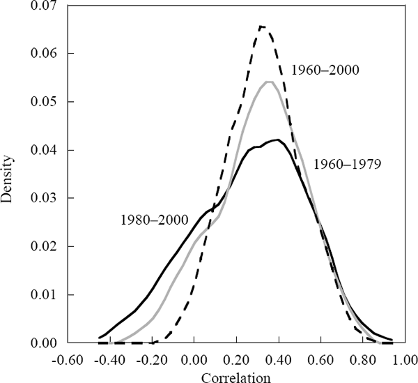
We can examine the stability of the bilateral correlations in two ways. First by plotting the correlations for the 1980–2000 sample against those for 1960–1979; this is reported in Figure 1. This figure indicates that there is a relatively weak (although statistically significant) positive relationship between the two sets of correlation measures. A second approach is to estimate the density function (essentially a smoothed histogram) for the estimated correlations over the full sample 1960–2000 and over the two sub-samples. All three densities are shown in Figure 2.[5] The most important difference between the density functions is that those for the sub-samples include more (and larger) negative correlations than the density function for the full sample. It would appear that the large negative correlations observed in the two sub-samples are only a transitory feature. Thus pairs of countries that are negatively correlated in one period tend to be positively correlated in the other period.
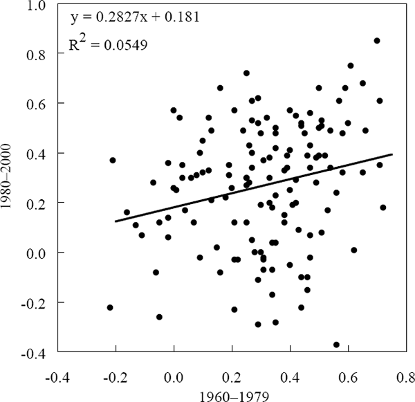
Neither Figure 1 or 2 can be taken as direct evidence that the changes in the international economic environment have altered the nature of the relationships between economies. For example, the changing pattern of correlations could reflect changing patterns of trade (if trade relationships were principally responsible for the correlation of GDP growth). Nonetheless, the weak relationship between the two periods that is indicated by Figure 1 suggests that it may be difficult to adequately model the complete sample. For this reason, we choose to focus our analysis on the latter sub-sample 1980–2000. This also has the advantage of providing information that is likely to be relevant to the current international economic environment.
Finally, to provide some further feel for the data, Figures 3 and 4 present the twenty most closely and least closely correlated pairs. Correlations for both the 1960–1979 and 1980–2000 period are reported; the correlations are ordered on the basis of the 1980–2000 sample.
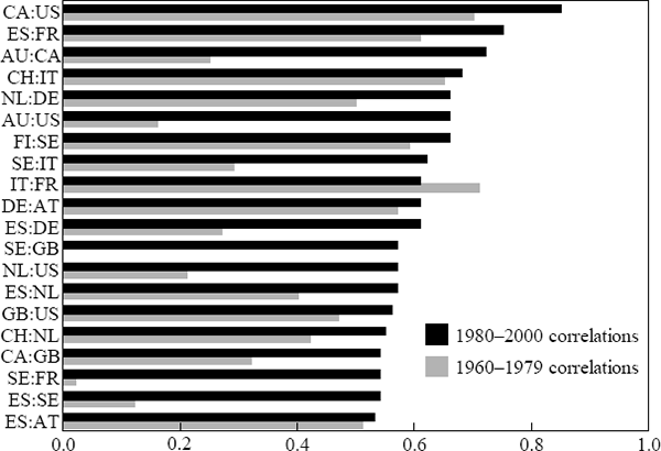
Note: See Table B1 for an explanation of country codes.
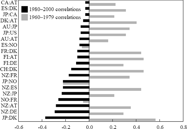
Note: See Table B1 for an explanation of country codes.
Not too surprisingly, numbered among the highly correlated economies are pairs of European countries, such as Spain (ES) and France (FR).[6] These countries are all quite closely integrated, both through trade and, for many, through common monetary policy, as well as many other European initiatives for greater economic and political integration that have come into force since the Treaty of Rome in 1957. Also, not too surprisingly, Canada (CA) and the United States (US) are the most highly correlated two economies in the 1980–2000 period (and the second highest in the earlier period). What is surprising is the fact that the correlation of Australia with the US (and by implication Canada) is among the highest of our group of countries. As we noted in the introduction, this high correlation is somewhat difficult to explain and is one of the motivations for the current study. It is interesting to note that this high correlation between Australia and the US is a feature only of the 1980–2000 period; for the earlier sample, the correlation is only 0.16.
The least correlated economies are presented in Figure 4. The two countries that appear most often in this regard are Japan (JP) and New Zealand (NZ). This probably reflects the unique events that these countries experienced over a considerable part of the sample period. In the case of New Zealand, the large structural reforms of the late 1980s and early 1990s; in the case of Japan, the stagnant growth that occurred in the wake of the bursting of the asset price bubble in the early 1990s. These two examples serve to highlight that idiosyncratic events can be influential and need to be borne in mind throughout the analysis. It also seems that country-specific shocks are not necessarily transmitted via trading links to other economies. While Japan is a major export destination for Australian goods, output growth in these two countries is virtually uncorrelated in the 1980–2000 period.
Table 1 also reports the correlations among the English-speaking economies of our sample: Australia (AU), Canada (CA), New Zealand (NZ), United Kingdom (GB) and United States (US). The strong correlation between GDP growth in Australia and the US has already been noted. In addition, other studies (for example Artis 2000) have noted a strong correlation between the US and UK business cycle, despite the close trade, financial and, at least until 1992, policy linkages of the UK with the European economies. From this, it seems useful to consider the English-speaking economies as a group.
For the full sample and the most recent sample, the mean correlation among the English-speaking economies is significantly higher than the mean correlation for all countries. The most dramatic difference occurs in the 1980–2000 sample. For this period, all of the correlations are positive, 0.22–0.85, and the mean correlation is nearly twice that of the full set of countries, 0.52 compared to 0.27. Interestingly, this strong relationship between these economies is not apparent in the 1960–1979 sample. Although the correlations are uniformly positive, the mean correlation is the same as that for the entire set of countries, 0.31.
The empirical models that we develop in this paper seek to explain the bilateral correlations for all of the countries in the sample. However, given our interest in Australia and the US, and the English-speaking countries more generally, we examine in some detail the ability of our model to explain the pattern of bilateral correlation that we observe for these countries.
Footnotes
See, for example, Dungey and Pagan (2000); de Brouwer and Romalis (1996); de Roos and Russell (1996); Debelle and Preston (1995) and Gruen and Shuetrim (1994). [1]
See Canova and Dellas (1993); Frankel and Rose (1998); Clark and van Wincoop (1999) and Imbs (2000). [2]
Canova and Dellas (1993) have a similar objective to this paper. Frankel and Rose (1998), in contrast, are concerned with a slightly different issue, whether or not highly correlated business cycles, a criteria for participation in a common currency, are a function of the extent of trade. If so, then participation in a common currency, by increasing trade, is likely to ensure that participating countries have highly correlated business cycles. [3]
We focus on growth rates of GDP as our means of identifying common cycles in the economies we consider. Growth rates have the advantage of being a natural measure of how economies perform over the cycle; however, they are not the only means of describing the business cycle and, in fact, they may be a poor measure of the business cycle for a variety of technical reasons, see Baxter and King (1995). Nonetheless, we believe that growth rates provide a reasonable and natural measure of the business cycle that is sufficient for our purposes. Some support for this is provided by Frankel and Rose (1998), who consider a variety of different means of detrending the GDP data, including four-quarter-ended growth rates as we do here, and find that the results are not very sensitive to the different detrending methods. [4]
The estimates were obtained with StataCorp (1997) and use a Epanechnikov kernel. [5]
An index of country codes is provided in Appendix B. [6]