RDP 1999-03: Householders' Inflation Expectations 4. The Structural Foundation of Inflation Expectations
January 1999
- Download the Paper 390KB
From Section 3, it is clear that there is a range of inflation expectations and that this range depends somewhat on the particular characteristics of the individuals involved. In this section, we explore the structural foundation underlying inflation expectations. Economists, of course, have their favoured models of the inflation process. The public, however, may have different ideas, and may systematise information in different ways to economists.
A 1996 study by Shiller comparing US, German and Brazilian survey data on the perceived costs of inflation confirms the differences in thinking between economists and the wider public. The public view the main problem with inflation as being the lowering of living standards because they do not perceive any compensating increase in nominal wages. The indirect costs of inflation commonly cited by economists, such as ‘shoe-leather’ and ‘menu’ costs and the uncertainty created by inflation, are generally not mentioned by non-economists. The general population is also concerned with psychological effects of inflation, believing that it is detrimental to national morale. In addition, the public often take little interest in the details of economic conditions. On average only about 3 per cent of respondents to the Melbourne Institute survey report being aware of inflationary developments, and just under one half of respondents cannot specify what type, if any, of economic news they have heard in the last few months.
In Section 4.1, we examine the responsiveness of individuals' inflation expectations to what the individuals themselves think will happen to some key macroeconomic variables and to the actual outcomes for a wider set of macroeconomic variables. In Section 4.2, we model the Melbourne Institute's published median of householders' inflation expectations.
4.1 A Cross-section Analysis
This section examines the structural foundation of householders' inflation expectations by examining the interaction of individuals' expectations with a range of economic information. Section 4.1.1 relates individuals' expected inflation to their expectations about the economy and the labour market, and to a series of general macroeconomic variables. The macroeconomic variables considered include past inflation, import price inflation, exchange rate movements, the output gap, the unemployment rate and interest rates. Section 4.1.2 looks at the interaction between individuals' wage and price expectations. The aim of this exercise is to see what sort of relationships people perceive between these variables.
The individual unit records on inflation expectations are analysed using cross-section techniques. This provides a data set of 28,356 observations in the full sample, and 23,370 in the 0 to 10 per cent sub-sample. (Respondents who have not answered all relevant questions have been excluded.) Since the respondents to the survey change each month, there is no continuity in respondents.
4.1.1 Responsiveness of inflation expectations to individuals' assessment of economic developments and actual macroeconomic outcomes
In this section, we examine how individuals' inflation expectations respond to expected and actual macroeconomic outcomes using unit record data from January 1995 to April 1998. Analysis is restricted to respondents whose inflation expectations are in the realistic range of 0 to 10 per cent, although the results are qualitatively similar when all responses are considered. Individuals' inflation expectations are regressed on individual characteristic dummies, dummies for individuals' expectations about unemployment and economic conditions in general, and macroeconomic variables commonly included in mark-up models of inflation. The regression results are presented in Table 4. Individual characteristic dummies relating to gender, age, occupation, education, political view, income and location are included in this regression but are not reported here. The results for individual characteristics are much the same as those presented in Table 2, where inflation expectations are regressed on individuals' characteristics only.
| Coefficient | Standard error | |
|---|---|---|
| Constant | −0.07 | 3.19 |
| Expected economic conditions: | ||
| Good | −0.52* | 0.06 |
| Qualified good | −0.59* | 0.06 |
| Some good, some bad | −0.34* | 0.05 |
| Qualified bad | −0.20* | 0.06 |
| Exclusion of expected economic conditions | F4,23,296 = 33.43* | |
| Expected unemployment: | ||
| More unemployment | 0.69* | 0.05 |
| Same unemployment | 0.28* | 0.05 |
| Exclusion of expected unemployment | F2,23,296 = 95.11* | |
| Four-quarter-ended underlying inflationt−1 | 1.83* | 0.38 |
| Unemploymentt−1 | −0.26 | 0.17 |
| Unemploymentt−3 | 0.61* | 0.18 |
| Unemploymentt−6 | −0.05 | 0.19 |
| Unemploymentt−9 | −0.39* | 0.18 |
| Unemploymentt−12 | 0.33 | 0.20 |
| Exclusion of lagged unemployment | F5,23,296 = 283.21* | |
| ΔUS dollart−1 | −0.03 | 0.02 |
| ΔUS dollart−3 | −0.04 | 0.03 |
| ΔUS dollart−6 | −0.05 | 0.03 |
| ΔUS dollart−9 | −0.02 | 0.03 |
| ΔUS dollart−12 | −0.01 | 0.03 |
| Exclusion of lagged three-month changes in US dollar exchange rate |
F5,23,296 = 0.59 | |
| Real cash ratet−1 | 0.14 | 0.16 |
| Real cash ratet−3 | −0.10 | 0.11 |
| Real cash ratet−6 | −0.06 | 0.10 |
| Real cash ratet−9 | −0.23* | 0.10 |
| Real cash ratet−12 | −0.05 | 0.14 |
| Real cash ratet−18 | −0.11 | 0.08 |
| Real cash ratet−24 | 0.01 | 0.06 |
| Exclusion of lagged real cash rate | F7,23,296 = 2.25* | |
Notes: * denotes significance at the 5 per cent level. The Wald F-statistic is presented for joint exclusion tests. |
||
The first shaded and unshaded blocks in Table 4 present the coefficients and standard errors for the dummies for respondents' opinions about economic and employment prospects respectively. Respondents are asked: ‘Thinking of economic conditions in Australia as a whole, during the next 12 months, do you expect we will have good times financially, or bad times, or what?’. They are then asked to provide an answer according to the scale: ‘good times’, ‘good times with qualifications’, ‘some good, some bad’, ‘bad times with qualifications’ and ‘bad times’. Respondents are also asked about employment conditions: ‘Now, about people being out of work during the coming 12 months. Do you think there will be more unemployment than now, about the same, or less?’. Respondents can answer according to the scale: ‘more unemployment’, ‘about the same or some more or some less’ and ‘less unemployment’.
The base case for expected economic conditions is ‘bad times’ and the base case for expected employment prospects is ‘less unemployment’. The coefficients on expected economic conditions are significant and negative, and the coefficients on expected unemployment are significant and positive. The better economic conditions are expected to be, the lower is inflation expected to be. The lower is expected unemployment, the lower is inflation expected to be. While not reported, the coefficients do not vary significantly by occupation grouping.
The relationship found between economic prospects and inflation has a straightforward explanation. The public associate ‘good times’ in the future with high output, low unemployment and low inflation, while ‘bad times’ are the opposite.[6] On the face of it, this suggests that people in fact expect to derive a direct benefit from price stability. This is consistent with Shiller's (1996) survey finding that the public views inflation as costly, both in economic terms and to national morale.
The rest of Table 4 shows how inflation expectations respond, on average, to aggregate macroeconomic variables. A straightforward way to model inflation is as a mark-up over unit labour costs and import prices in domestic currency, with the mark-up varying over the course of the cycle (de Brouwer and Ericsson 1998). This suggests that the matrix of key macroeconomic variables which are possible ‘fundamental’ explanators of inflation expectations includes past inflation, wages growth, import price inflation, exchange rate movements, the output gap (defined here as the deviation of output from a Hodrick–Prescott trend from 1980 to 1997) and the unemployment rate. We also include the real cash rate (calculated as the nominal cash rate less inflation over the past year) in order to capture direct effects of monetary policy changes on inflation expectations. Quarterly data are interpolated on a monthly basis where necessary.[7]
Table 4 provides some indicative results, with lags of the real cash rate, the unemployment rate and the three-month change in the Australian/US dollar exchange rate included as explanatory variables.[8] There are three main results. The first is that most of the key macroeconomic variables do not explain householders' inflation expectations. Inflation expectations do not systematically respond to exchange rate movements, import price changes, wages growth or the output gap at any lag length. While lags of the unemployment rate are jointly, and sometimes individually, significant, the sum of the coefficients on these lags is positive. The second result is that past inflation is an important explanator of expected inflation, with a coefficient of 1.83.[9] When insignificant variables are excluded, the coefficient on past inflation is numerically very close to 1.0 and not significantly different from it.
The third result is that monetary policy has a systematic and robust effect on inflation expectations. The interest rate is defined as the real cash rate – the nominal cash rate less inflation over the past year – but the outcome is qualitatively similar when the nominal cash rate or the nominal or real mortgage interest rate is used. The cash rate at the end of the previous month has a positive impact on inflation expectations, but other lags, up to 18 months out, have a negative effect on inflation expectations. The net direct effect of a rise in the real cash rate is negative, with the sum of the coefficients being −0.4. While only the nine-month lag of the real cash rate is individually significant, all lags are jointly significant. The individual significance of lags increases when other insignificant variables are excluded.
4.1.2 The interaction of expected changes in wages and prices
The Melbourne Institute periodically asks householders additional questions. One such question, asked since March 1997, has been about respondents' expected wage increases over the coming year. Interviewers ask respondents: ‘Turning now to the wage or salary you expect to receive for your job. Do you think that your average hourly rate of pay is likely to increase, decrease or stay the same over the coming 12 months?’. While people would anticipate that their wages may rise for a number of reasons, the desire to at least maintain real wages should mean that, in general, people tend to expect their wages to rise at least as much as they expect prices to rise.
We find, however, that there is no systematic relationship between what an individual expects to happen to their wages growth and inflation, even after controlling for method of wage determination. While we do not report the results of the regressions (which show a negative but insignificant correlation), Figure 5 is a three-dimensional graph showing expected inflation, expected wages growth and the relative frequency of these responses as at May 1998. The sample is restricted to respondents who expect rises in both of these variables to be between 0 and 10 per cent. The range of expected wage changes does not match the range of inflation expectations. Most people whose inflation and wage change expectations lie between 0 and 10 per cent expect no change in their wages, regardless of their inflation expectations.
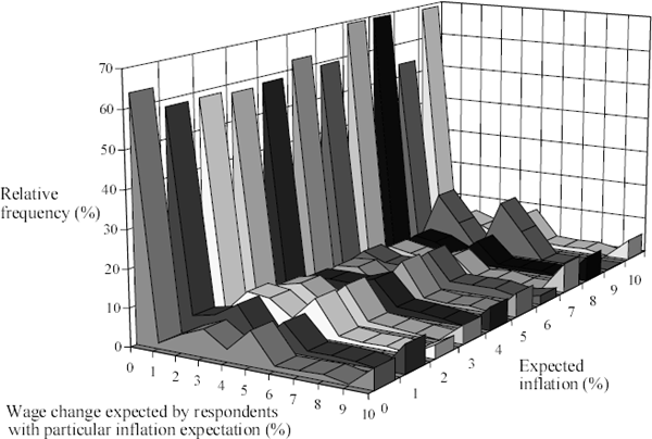
This result accords with Shiller's (1996) survey finding that the general public does not believe that inflation is matched by compensating increases in nominal wages. People may believe that it takes some time for price rises to be reflected in wages, or alternatively, they may think that there are other factors which are more important in determining wages.
4.1.3 Summary of cross-section analysis
The cross-section analysis of individuals' answers to the survey on inflation expectations provides two broad insights. First, and unsurprisingly, the public's view of economic relationships differs materially from that of economists. For example, they associate good economic conditions with low unemployment and low inflation, rather than anticipating higher inflation when the economy is growing more strongly and facing greater supply constraints. Similarly, they do not systematically expect exchange rate or wages movements to affect inflation. At least from the results here, it appears that people do not expect their wages to grow in line with what they expect to happen to prices.
The second interesting result is that inflation expectations move with recent inflation and respond to monetary policy. While a tightening of monetary policy is initially associated with a rise in inflation expectations (perhaps because the tightening is a strong signal of higher future inflation), the overall impact of a policy tightening is to lower inflation expectations. This is a robust result. There is a direct, negative, significant and lagged effect of monetary policy on inflation expectations.
4.2 Explaining Householders' Median Inflation Expectations
Data on householders' median inflation expectations are considerably more accessible and easier to use than those on individual householders' inflation expectations. In this section, we carry the analysis conducted in Section 4.1 on individuals' expectations over to householders' median inflation expectations, examining how median expectations are influenced by a range of macroeconomic variables.
In the unit record analysis in Section 4.1, cross-sectional regression was conducted. When the focus is on the median, however, the cross-sectional aspect is lost but the time dimension is gained. Using time-series techniques introduces three challenges. First, there is the issue of non-stationarity in inflation expectations. As is clear from Figure 1, there has been a mean change in both inflation and inflation expectations from the 1980s to the 1990s. The series may be non-stationary, with the attendant econometric problems. One way to deal with this is to restrict the statistical analysis to the new ‘regime’, basically from 1992; another is to use cointegration techniques. Second, in the cross-section analysis there was a surfeit of degrees of freedom but this is not the case in the time domain, especially if the sample period is truncated to the low-inflation period of the 1990s. This means that parameter estimates are less precise. Third, given that the dependent variable is inflation expected over the coming year, monthly or quarterly regression analysis of this variable will induce a moving-average process in the residuals. This is corrected using the procedure outlined in Newey and West (1985) (using the robusterrors option in RATS).
Presuming that inflation is a possibly time-varying mark-up over costs, variables relevant in explaining inflation expectations would include unit labour costs, wages, import prices, exchange rates (either multilateral TWI indices or bilateral with the US dollar), the output gap and the unemployment rate. As it turned out, consistent with the unit record analysis in the previous section, none of these macroeconomic variables were found to have a systematic – or indeed any – effect on the median inflation expectation. This was examined over a number of sample periods. We started regression analysis from January 1992, a period over which inflation and inflation expectations are mean reverting. An error-correction specification was also used to examine the relationship between inflation expectations and macroeconomic variables in periods extending back to the 1980s. We tried starting the estimation from January 1987, the time when the survey went monthly. Quarterly observations back to 1980 were also experimented with.[10] None of these forays into the data revealed a systematic effect of macroeconomic variables on householders' median inflation expectations. The results are not reported here, but are available on request.
As in the previous section, interest rates were also included in the analysis, and the cash rate, either nominal or real, repeatedly emerged with a significant and negative sign.[11] The six-month lag of the real cash rate emerges as the key explanator (which is the second lag when the equation is estimated on a quarterly basis). The real rate is calculated as the nominal rate less the Melbourne Institute measure of expected inflation, although the results are qualitatively similar when the real rate is calculated as the nominal rate less actual inflation over the past ayear. A similar story emerges when the models include the nominal cash rate, since changes in nominal cash rates are dominated by changes in the real rate.
We provide a few representative examples in Table 5. Model 1 states that expected inflation depends on past actual[12] and expected inflation, and falls as monetary policy is tightened. This estimate suggests that inflation expectations directly fall by 0.1 per cent for a 1 per cent tightening of monetary policy six months earlier, with a long-run direct effect of ¼ per cent. Models 2 and 3, which are in error-correction format, model expected inflation over progressively longer sample periods, and indicate that inflation expectations fall by up to 0.4 per cent for a sustained 1 per cent tightening in policy. These estimates relate only to the direct effect of policy changes on inflation expectations; changes in policy also affect inflation, directly through the exchange rate and indirectly through the output gap. Changes in inflation in turn affect expected inflation, implying that the total effect is greater. It may seem somewhat puzzling that people's inflation expectations respond several months after policy changes. However, we find this result both in the regressions explaining individuals' inflation expectations, reported in Section 4.1, and in the regressions explaining median inflation expectations.
| Model 1 Dependent variable: inflation expectations  |
Model 2 Dependent variable: change in inflation expectations  |
Model 3 Dependent variable: change in inflation expectations  |
||||
|---|---|---|---|---|---|---|
| Monthly January 1992–May 1998 |
Monthly January 1987–May 1998 |
Quarterly March 1980–June 1998 |
||||
| Coefficient | Standard error | Coefficient | Standard error | Coefficient | Standard error | |
| Constant | 1.07* | 0.14 | 0.23 | 0.12 | 0.25* | 0.12 |
 |
0.56* | 0.05 | −0.13* | 0.05 | −0.10 | 0.06 |
| πt-1 | 0.44* | 0.05 | 0.16* | 0.06 | 0.10 | 0.06 |
| Real ratet-6 | −0.11* | 0.04 | −0.04* | 0.01 | – | – |
| Real ratet-2 | – | – | – | – | −0.03* | −0.01 |
 |
0.56 | 0.09 | 0.06 | |||
| α1 + α2 = 1 | χ2(1) = 2.05 | – | – | |||
| β1 = β2 | – | χ2(1) = 4.01* | χ2(1) = 0.51 | |||
Notes: * denotes significance at the 5 per cent level. When estimating from 1987 and 1992, degrees of freedom problems require monthly observations to be used, thus CPI figures must be interpolated. When estimating from 1980, the sample period is sufficiently long to allow quarterly observations to be used. The restriction that expected inflation is a homogeneous linear function of actual and expected inflation is not rejected at the 5 per cent level and is imposed. The restriction that actual and expected inflation move one-for-one in the long run is not rejected at the 5 per cent level when the sample period starts in 1980 and is imposed. This restriction is rejected when estimating from 1987 onwards. When the real cash rate is alternatively defined as the nominal cash rate less actual inflation over the past year, however, this restriction is not rejected and its imposition yields results similar to those presented above. |
||||||
4.3 Rationality of Expectations
The finding that householders' inflation expectations do not take into account variables included in structural models of inflation may suggest that expectations are not formed rationally. In this section we test whether expectations are unbiased and whether they are efficient in the sense that they use all available information. The standard test for bias is whether α equals zero and β equals 1 in Equation (1):

The results from estimating this equation for quarterly Australian data, starting from March 1980 and March 1992, are presented in columns 1 and 2 of Table 6. The dependent variable is the inflation rate four-quarters ahead so that actual and expected inflation refer to the same period. The joint hypothesis that α and β equal 0 and 1 respectively is rejected for both sample periods. In accordance with findings in de Brouwer and Ellis (1998), the restriction that β equals 1 cannot be rejected on its own when the sample period starts in 1980. Although inflation expectations are biased, they move one-for-one with actual inflation over this sample period.
Estimated equation
|
Estimated equation
|
|||||||
|---|---|---|---|---|---|---|---|---|
| March (Q) 1980– June (Q) 1997 |
March (Q) 1992– June (Q) 1997 |
March (Q) 1980– June (Q) 1997 |
March (Q) 1992– June (Q) 1997 |
|||||
| Coeff. | Std error | Coeff. | Std error | Coeff. | Std error | Coeff. | Std error | |
| Constant | −2.27* | 0.62 | −1.02 | 1.58 | 0.16 | 3.00 | 0.12 | 1.14 |
 |
1.01* | 0.12 | 0.76 | 0.41 | 0.84* | 0.30 | 1.09* | 0.33 |
| πt-1 | – | – | – | – | 0.08 | 0.28 | −0.69* | 0.21 |
| Unempt-1 | – | – | – | – | −0.20 | 0.27 | −0.08 | 0.08 |
| ΔUS dollart | – | – | – | – | −0.06* | 0.03 | 0.01 | 0.01 |
 |
0.77 | 0.19 | 0.78 | 0.45 | ||||
| β=1 | χ2(1)=0.02 | χ2(1)=0.33 | – | – | ||||
| (α,β)=(0,1) | χ2(2)=86.37* | χ2(2)=175.03* | – | – | ||||
Notes: * denotes significance at the 5 per cent level, π indicates annual rate of inflation. |
||||||||
In economists' jargon, the rationality of expectations implies that people use all available information to form their expectations. Columns 3 and 4 of Table 6, however, indicate that, at least in the simple framework of Equation (1), householders do not systematically use all available information: by using available information about inflation and the exchange rate, they could improve their inflation forecasts. In other words, the error term in Equation (1) is supposed to be a white noise process, but in fact, it exhibits systematic behaviour related to past inflation and the six-month change in the exchange rate.
Footnotes
This result is robust to the exclusion of the macro variables in the regression. [6]
Using quarterly data gives qualitatively similar results. [7]
Including lags of variables as regressors does not necessarily imply that expectations are backward looking. Just as economists use past information to forecast variables into the future, forward-looking individuals may similarly use past information to form their expectations. [8]
In the regressions presented above, inflation refers to the growth in the Treasury underlying CPI. Given that respondents are asked what they expect to happen to the prices of things they buy, other measures of inflation may be more relevant. Changes in the CPI excluding interest and volatile items, or excluding interest and consumer credit charges, may be closer approximations to what people have in mind when thinking about changes in prices of the things they buy. These measures of past inflation also have significant and positive effects on inflation expectations. [9]
Within this period we also tested for the effect of large exchange rate movements, defined as a 5 or 10 per cent change, on the median expectation. [10]
We use the target cash rate from 1990 onwards and the unofficial cash rate before then. [11]
In the results presented in Table 6, actual inflation is measured using the Treasury Underlying CPI. The CPI excluding interest and volatile items, which may better reflect the prices of things people buy, gives qualitatively similar results. The CPI excluding interest and consumer credit charges has no significant effect on inflation expectations. [12]