RDP 9810: The Distribution and Measurement of Inflation 3. Measuring Core Inflation
September 1998
- Download the Paper 326KB
In a closed economy, core inflation is typically regarded as being the persistent component of inflation, the rate of change of prices that is caused by the interaction of aggregate demand and supply (Blinder 1982; RBA 1994). In an open economy, like Australia, sustained movements in the exchange rate will also affect the persistent component of inflation. However, measured inflation can differ markedly from such a definition of core inflation. The published series may reflect shocks to the supply of particular goods or services and, over short horizons, it may exhibit a seasonal pattern. Statistically, like other time series, inflation can be decomposed into trend, irregular and seasonal components. The trend component equates to the economic concept of core inflation. However, several methods exist for defining and removing irregular and seasonal components, and so constructing measures of core inflation.
3.1 Methods for Measuring Core Inflation
To be widely accepted, and to be useful for economic policy purposes, a measure of core inflation should be easily understood, available on a timely basis, not subject to revisions, and capable of being easily verified (ABS 1997a; Roger 1997). Broadly, three methods are used to construct measures of core inflation: certain components can be regularly excluded; there can be case-by-case specific adjustment of prices; or, some statistical criterion can be used.
Exclusion-based measures of core inflation permanently remove specified components from the CPI basket because their price movements over a short horizon are perceived to be unrepresentative of market-induced inflation trends. Typically, their prices are: seasonal; volatile, so movements are often quickly reversed; or largely determined by government policy. The Treasury underlying CPI used in Australia, and the CPI excluding food and energy in the US, are both exclusion-based measures of core inflation. Such measures are timely and transparent. They are also relatively intuitive and easily understood, although these advantages decline if a large proportion of the basket is excluded. Exclusion-based core inflation measures do have significant limitations. Information is discarded with the price changes of the components that are excluded. Further, it is necessary to make an ex ante judgment on which components to exclude. If the excluded components have a different trend rate or cyclical pattern of inflation, an exclusion-based core series may be somewhat unrepresentative of general price movements. Finally, an exclusion-based approach does not control for shocks to components retained in the basket.
Specific-adjustment methods of calculating core inflation are conceptually preferable to other methods, because by definition, they measure only those price movements attributable to the balance of supply and demand. In each period, the estimated impact on each component of changes in taxes and subsidies, seasonality and volatility are removed, with the residual price changes for all components combined to produce the core inflation series. While such a series defines the concept of core inflation well, it requires a large amount of information, and judgment, to decompose the price movements for each component into core and non-core changes. As such, it is less timely and cannot be easily verified, so is unlikely to be widely understood or accepted.
Statistical measures (or limited-influence estimators) of core inflation remove, or reduce the weight of, those components with extreme price changes, based on the premise that extreme price changes are not indicative of the persistent component of inflation. The most common class of these measures is the trimmed mean. These measures remove a proportion of each tail of the distribution, and take the weighted average price change of the central core of the distribution. They are timely and highly transparent, with no judgment required for their construction once the size of the trim is specified (although they may be more difficult to communicate to a broad audience than exclusion based core measures). Trimmed means have been calculated for many countries.[11]
The best known trimmed mean is the 100 per cent trim centred at the midpoint of the distribution. This is, of course, the median: the price change of the central component of the distribution. In principle, however, a 100 per cent trimmed mean can be ‘centred’ anywhere in the distribution. (For example, the 100 per cent trim centred at the 52nd percentile measures the price change of the component ranked at the 52nd percentile in the distribution.) To anticipate the results, it is found that a 100 per cent off-centre trimmed mean is often the ‘optimal’ measure of core inflation.
It may seem odd that an ‘optimal’ measure of core inflation could be derived by focusing solely on the price change of one component of the distribution. However, it should be remembered that the rest of the distribution is not simply ignored in the calculation of a 100 per cent trimmed mean. Instead, all price changes are ranked from the lowest to the highest, and the price change of the component at the chosen percentile of the distribution is recorded.
3.2 Distributions and Statistical Measures of Inflation
Section 2 demonstrated that the cross-section of price changes frequently contained outlying observations, in one or both of the tails of the distribution. Such extreme price changes greatly affect the mean rate of inflation. Furthermore, they are typically unrepresentative of the trend rate of inflation.
The components that Department of Treasury (1995) classify as having volatile or seasonal prices, or prices that are heavily influenced by government policy, are excluded from the Treasury underlying measure of inflation. These components are among those most often found in the tails of the distribution although they are not always in the tails (as Appendix B shows). Also, items retained in exclusion-based core inflation measures are occasionally in the tails of the distribution. If extreme price changes are unrepresentative of the persistent component of inflation, an exclusion-based measure of core inflation will often include unrepresentative price changes but exclude valuable information. Trimmed means, in contrast, may be a better measure of core inflation because they remove extreme price changes regardless of the nature of the component that experiences that price change.[12]
As noted, the mean inflation rate is heavily influenced by how far in the tails is an extreme price change. In contrast, for trimmed mean measures of inflation, the ranking of extreme price changes is relevant, not their distance from other price changes; for the remaining central core of components, their distance from other price changes, and not just their ranking, is important in determining the trimmed mean rate. However, for the median measure of inflation, all component price changes are treated equally; only the ranking of each component price change is relevant in determining the value of the median.
3.3 Constructing a Statistical Measure of Core Inflation
Statistical measures of core inflation can be calculated using component price changes over any horizon. In this paper, they are all based on quarterly changes – the shortest horizon possible with Australian CPI data – as such series should provide more timely information on turning points in inflation. In addition, because the components excluded change each quarter, components that are subject to a large price shock need only be excluded for one period rather than several. This section outlines how the preferred trimmed mean might be chosen.
As discussed above, the high leptokurtosis of the distribution of price changes implies that there are many observations in the extremities of the tails which have a disproportionate influence on the mean. Indeed, as the degree of excess kurtosis increases – implying there are more price changes that are unrepresentative of the core rate – it may be desirable to remove a larger proportion of the tails of the distribution in calculating a trimmed mean measure of inflation. Particular attention must be given to the skew of the distribution when constructing a trimmed mean measure of inflation. If the distribution is, on average, positively skewed, observations in the right-hand tail will typically be further from the mean than the observations in the left-hand tail. Hence, if the trim is symmetric – that is the same proportion is removed from both tails – the trimmed mean will systematically record lower inflation than the sample mean. Conversely, for a negatively skewed distribution, a symmetric trimmed mean will record higher inflation than the sample mean.
Given the systematic positive skew of the distribution of CPI component price changes, there is likely to be a bias in the average inflation rate of a symmetric trimmed mean. This bias can be eliminated by removing a larger proportion of the trim from the tail opposite to the direction of the skew, i.e. from the left-hand tail. The larger is the average coefficient of skewness the larger is the proportion of the trim that must be taken from the left-hand tail to avoid average rate bias.
Since theory prescribes neither the optimal size of the trim, nor the extent to which it should be asymmetric, a benchmark is needed to compare the range of trimmed means. This paper examines how closely various trimmed means track a proxy for the trend, or persistent, component of inflation. The range of trimmed means can be compared using the mean absolute deviation (MAD) and root-mean-squared error (RMSE) between the trimmed mean quarterly rate of inflation and the proxied trend series. The MAD penalises all deviations from the trend series equally, while the RMSE places a higher penalty on those deviations further from the trend.
Bryan, Cecchetti and Wiggins (1997) use a 36-month-centred moving average of the mean inflation rate as a proxy for the trend component of US CPI inflation. Higher import penetration, and the resultant dependence of the CPI on exchange rate movements, suggests that the Australian CPI is likely to demonstrate considerably less inertia than the US CPI, so that a shorter moving average may be more appropriate. Since the exact length of the moving average that best represents the trend component of inflation remains unknown, however, this paper uses several moving averages. Several Hodrick-Prescott filters of the quarterly mean inflation rate are also used to proxy the trend component of inflation. Hodrick-Prescott filters have the advantage that for relatively large smoothness parameters, they will be affected less by a one-off shock to the mean inflation rate.
3.4 Comparing Trimmed Means
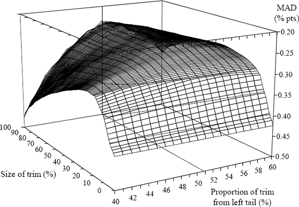
Figure 3 presents a comparison of trimmed means against an initial benchmark. It plots the MADs for a range of trimmed means from a five-quarter-centred moving average of total CPI inflation. The side axis shows the size of the trim, ranging from 0 (the total CPI basket is retained) to 100 (a complete trim). In the latter case, the trimmed mean rate of inflation is the price change for the component that covers the given percentile. If that percentile is the 50th, the trimmed mean is the weighted median rate of inflation.[13] The front axis shows the proportion of the trim taken from the left-hand tail. Only the range from 40 to 60 per cent is shown because, outside this range, large trimmed mean rates of inflation differ markedly from the moving average rate of inflation. The vertical axis shows the inverted MAD for each of the trimmed means from the moving average. By the chosen criteria, the smaller the MAD for a given trimmed mean, the better that series performs as an indicator of core inflation. The MAD is reduced substantially by trimming even a small proportion from the tails, so providing a better measure of core inflation. While the incremental gain from increasing the size of the trim beyond around 50 per cent declines rapidly, it is nonetheless positive.

For a given size trim, the MAD is smallest when more of the trim is removed from the left- than the right-hand tail. The need to trim asymmetrically arises because the distribution of price changes is, on average, positively skewed. The smallest MAD from a five-quarter moving average of the CPI quarterly inflation rate occurs for a 100 per cent trim, with 51 per cent of the trim from the left-hand tail. This trimmed mean – the price change of the component at the 51st percentile of the distribution of price changes in each quarter – reduces the MAD relative to the mean rate of inflation by 43 per cent.
The RMSE from a five-quarter moving average declines even more sharply than the MAD for very small trims. Like the MAD, the RMSE falls monotonically as the proportion trimmed increases. The skew of the distribution again leads to the 51st percentile (a 100 per cent trim) being the preferred trimmed mean. The RMSE from the moving average rate of inflation for the 51st percentile rate of inflation is 48 per cent lower than for the mean rate of inflation.
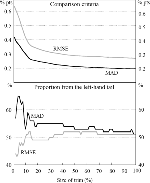
The sensitivity of the result to the use of a five-quarter moving average of quarterly inflation can be tested using different lengths of moving averages. Both seven- and nine-quarter moving averages, using the MAD and RMSE, show that there are significant gains to removing even a small proportion from the tails of the distribution. The top panel of Figure 4 shows the smallest MAD and RMSE for each size trim from a seven-quarter moving average, while the lower panel shows the proportion taken from the left tail for each of those trimmed means.

Again, after large decreases in the average deviation from the trend term for small trims, larger trims continue marginally to improve the measure of core inflation. Using the longer moving averages, the optimal trims are either 100 per cent or around 90 per cent. The seven- and nine-quarter moving averages derived trimmed means centred on the 51st and 52nd percentiles.
Because a centred moving average contains past values of inflation, its use to proxy trend inflation could possibly derive a trimmed mean that is not a timely indicator of turning points in inflation. To assess the nature of the trimmed means that provide the best indicators of turning points in inflation, a leading moving average can be used to compare the trimmed means. When the five-quarter moving average is shifted forward one or two quarters, the preferred trimmed mean based on both the MAD and RMSE is always large (again around 90 to 100 per cent) and typically centred on a percentile higher than the 50th. The finding that asymmetric trimmed means which remove a large proportion of the distribution perform best as estimators of core inflation therefore seems robust to the use of a leading moving average.
An alternative proxy to moving averages for the trend component of inflation is a Hodrick-Prescott filter of inflation.[14] Hodrick-Prescott filters have the advantage that the trend proxy will be influenced less by a one-off shock to the mean rate of inflation. Three smoothness parameters (λ = 5, 50 and 200) are used that produce plausible proxies for the trend component of inflation.[15] Again the MAD and RMSE of the trimmed means against the Hodrick-Prescott filtered inflation series is used to compare the trimmed means. Once again, large trimmed means (typically close to 100 per cent, but occasionally around 80 per cent), centred on the 52nd and 53rd percentiles track the trend proxy most closely.
The size of the optimal trim, and its asymmetry, may also differ episodically as the dispersion and skew of the distribution change. In particular, the rate of inflation has been lower in the 1990s, while the distribution of price changes has also been less dispersed and less skewed, but slightly more leptokurtotic. Using the RMSE and MAD calculated only from September 1990 as the criteria for judging the optimal size of the trim, it is still found that a large trim, in the range of 90 per cent, is the best representation of the trend component of inflation. Surprisingly, however, over the more recent period, the optimal trim is centred on a higher percentile – around the 54th percentile – than that based on the full sample.
3.5 Trimmed Means Based on Seasonally Adjusted Data
The trimmed means that performed best at capturing the trend in inflation in the previous section were all centred on a percentile higher than the 50th. This occurs because, as noted in Section 2.3, the distribution of component price changes is usually positively skewed. This skew is caused, in part, by the seasonal pattern of the price changes of some components, in particular the policy affected components. The need to centre trimmed means on a percentile higher than the 50th may be avoided by seasonally adjusting the component price changes.[16] Further, seasonally adjusting the price changes may reduce the extent to which the tails need to be trimmed.
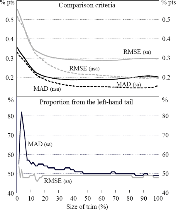
Seasonal patterns tend to evolve over time. As a result, ex post seasonal adjustment is likely to produce a smoother series than seasonal adjustment conducted contemporaneously. To make a fair assessment of the benefits of using seasonally adjusted data, the seasonal factors for each of the CPI components were projected one year out each June, from 1990 onward.[17] Trimmed means calculated from seasonally adjusted price changes were then compared using the MAD and RMSE from a five-quarter moving average from September 1990 onward. Seasonal adjustment reduced both the size and the asymmetry of the trim that minimised the MAD and RMSE. As Figure 5 demonstrates, for nearly all size trims, however, the trimmed means calculated using original data outperform those based on seasonally adjusted data, particularly for those with the lowest RMSE and MAD.

3.6 Choosing the Statistical Core Inflation Series
Using a range of criteria it was shown above that trimmed means that remove a large portion of the tails significantly outperform the sample mean, and smaller size trimmed means, as measures of the trend component of inflation. This result was invariant to the use of a Hodrick-Prescott filter or a moving average to proxy trend inflation, the length of the moving average, whether it was centred or leading, and the time over which the comparison is made. After substantial gains from trimming the initial half of each tail of the distribution, the gains from removing a larger proportion are small. The RMSE and MAD for the 50 per cent trim are no more than 10 per cent greater, about 0.02 percentage points, than the minimum RMSE and MAD trims. However, for most of the criteria used, the 100 per cent trimmed mean outperforms other size trims. The 100 per cent trim is also more intuitive in that it treats all price changes in the same manner.
Because the shape of the distribution may change periodically, any one trimmed mean may not always be the best representation of core inflation. This section develops two trimmed means, the 100 per cent trimmed mean, which is the optimal trimmed mean against many of the criteria used, and the 50 per cent trimmed mean. To increase the acceptance and usefulness of the trimmed means, it is desirable that the average rates of inflation measured by these core series and the full CPI basket are the same.
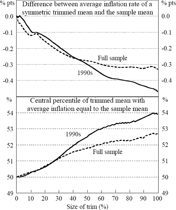
As Figure 6 demonstrates, the greater the size of the trim, the larger the bias in the average rate of inflation of a symmetric trim relative to the sample mean. As the size of the trim increases, it must be centred on a higher percentile to avoid the bias in the average rate of inflation. The average rates for the 50 per cent and 100 per cent trimmed means, centred on various percentiles, are shown in Table 3. The 50 per cent trimmed mean centred on the 52nd percentile records the same average rate of inflation as the sample mean over the full sample period and the 1990s. The 100 per cent trimmed mean must be centred slightly higher, on the 53rd percentile, to record average inflation equal to the sample mean over the full sample. The MAD and RMSE for the 100 per cent trimmed mean, from a five-quarter moving average, are 43 and 48 per cent lower than for the sample mean; for the 50 per cent trim, they are 41 and 45 per cent lower.

| Mean | Central percentile | ||||||
|---|---|---|---|---|---|---|---|
| 50th | 51st | 52nd | 53rd | 54th | 55th | ||
| 50 per cent trimmed mean | |||||||
| Sep 1980 to Mar 1998 | 5.5 | 5.2 | 5.4 | 5.5 | 5.7 | 5.8 | 6.0 |
| Sep 1990 to Mar 1998 | 2.8 | 2.5 | 2.6 | 2.8 | 2.9 | 3.0 | 3.1 |
| 100 per cent trimmed mean | |||||||
| Sep 1980 to Mar 1998 | 5.5 | 5.2 | 5.3 | 5.4 | 5.5 | 5.6 | 5.8 |
| Sep 1990 to Mar 1998 | 2.8 | 2.4 | 2.5 | 2.6 | 2.7 | 2.8 | 3.0 |
While the average rate of inflation of trimmed means centred on various percentiles differs, trimmed means of the same size centred close to each other exhibit virtually identical quarterly movements. Thus, while the ideal percentile on which to centre a trimmed mean may vary marginally over time, all trimmed means of the same size centred within an appropriate region identify identical turning points.
Footnotes
Several papers that outline the construction of trimmed means for various countries are Bryan, Cecchetti and Wiggins (1997), Bryan and Cecchetti (1994), Laflèche (1997), RBA (1994), Roger (1995) and Shiratsuka (1997). [11]
Bryan, Cecchetti and Wiggins (1997) argue in favour of trimmed means on the grounds that CPI component price changes are random draws from a population that is not normally distributed. Hence, as an estimator of the economy wide inflation rate (the population mean), trimmed means will be more efficient – that is, have smaller variance – than the sample mean. However, the components of the CPI are fixed and priced throughout the quarter, and so are not usually regarded as being random draws. [12]
Note, alternatively the median can be calculated as the weighted average of inflation rates from adjacent components in the distribution as demonstrated in Appendix C. [13]
The Hodrick-Prescott filter is developed in Hodrick and Prescott (1997). [14]
The smaller λ, the closer the filtered series tracks the actual series. [15]
Alternatively, the trimmed mean could be calculated on the basket excluding policy affected components, which is less skewed. However, since the price changes of these components often contain valuable information on inflation it is preferable to retain them in the basket. [16]
All seasonal adjustment was conducted using EZ-X11. [17]