RDP 9809: Estimating Output Gaps 2. Methods of Estimating the Output Gap
August 1998
- Download the Paper 387KB
The output gap is defined as the difference between actual and potential output:

where gap is the output gap, y is output and yT is potential output. In this form, a positive number for the gap indicates excess demand and a negative number indicates excess capacity. The output gap represents transitory movements from potential output. Given that potential output is not observed, it has to be estimated. Not surprisingly, different assumptions about potential output and different estimation methodologies yield different estimates of the output gap.
The role of the output gap in affecting wage inflation was shown by Phillips (1958). In empirical work, inflation is often characterised as a mark-up over unit labour costs and imported goods prices, with the mark-up varying over the business cycle (de Brouwer and Ericsson 1995). Wages growth, in turn, also appears to be sensitive to the state of the business cycle and the rate of economic growth (Cockerell and Russell 1995; de Brouwer and O'Regan 1997; Debelle and Vickery 1997). This indicates that the output gap contains valuable information about movements in price and wage inflation. From a policy perspective, however, the underlying trend or potential output component should be defined in terms of a non-accelerating (or decelerating) inflation rate. While several of the simple measures examined do not do this, the multivariate and production function approaches can provide an estimate of the output gap consistent with unchanging inflation.
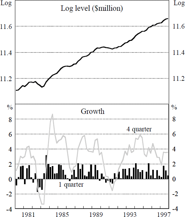
In this paper, output is defined as GDP(A), the broadest available measure, and is in 1989/90 prices. Figure 1 shows the log level and one- and four-quarter-ended growth rates of output from March 1980 to December 1997. This sample period excludes the growth slowdown that followed the oil price shocks in the 1970s, and so eliminates an important structural break. It indicates that the economy contracted in 1982/83 and in 1990/91, with the former recession being deeper but the latter more protracted. These two periods would be expected to be associated with negative output gaps with similar features. We now review various methods of estimating output gaps.
2.1 Linear Method
The simplest way to estimate the output gap is to calculate potential output using a linear trend, which, when estimated using logged quarterly GDP(A) from 1980 to 1997, yields the following equation:
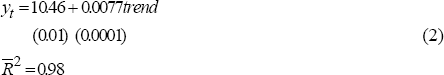
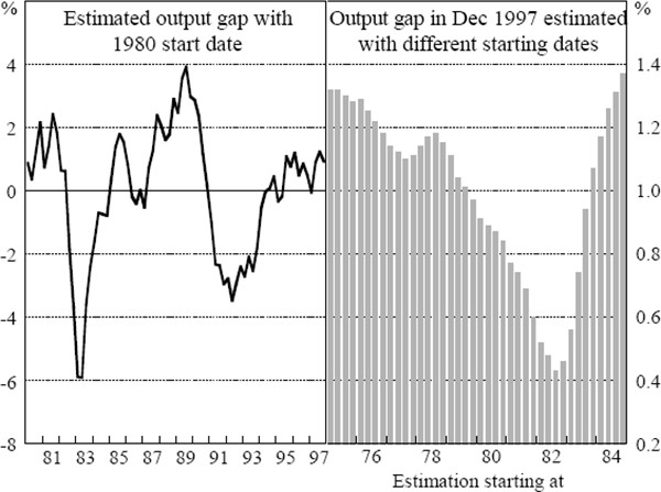
This estimates trend growth in output over the past couple of decades to be about 3.1 per cent a year. The output gap implied from this trend estimate is shown in the left-hand panel of Figure 2. The gap profile will be discussed in Section 3. A general criticism of this method (and one which also applies to other techniques) is that the estimate of the gap depends on the sample period. For example, the bars in the right-hand panel of Figure 2 show the estimated output gap for the last period in the sample – the December quarter 1997 – as the starting date for the estimation moves forward in time from March 1975 to December 1984. Output is estimated to be above potential at December 1997 for all the sample lengths examined, but the spread in the range of estimates is one per cent. The selection of starting and end-points in a linear regression matters. For example, when the sample starts at the lowest point in a recession, which is 1982 here, the slope of the straight line fitting the series is steeper, making the gap between actual and potential output at the end of the sample smaller. This highlights the importance of starting the regression at a period when the economy is basically in balance. The sensitivity of gap estimates to the sample period also underscores the general uncertainty of gap estimates.
The assumption that potential output grows at a constant rate is also difficult to accept. Output growth can be decomposed into growth of labour productivity and of labour inputs, which in turn can be decomposed into changes in population, labour force participation and average hours worked. There is no compelling reason for these components to be constant over time, especially when an economy has undergone considerable structural reform, and so a more general, time-varying, approach is preferable.
This is also reflected in the time series properties of the gap estimate. If output follows a deterministic trend, then the residual from removing that trend should be a stationary series. But if output is an integrated series of order one, and hence follows a stochastic trend, then the residual from removing a linear trend is still non-stationary. This would violate the usual assumption that the output gap is a mean-reverting variable, such that ‘shocks’ to it do not persist. There is a large and mixed literature on whether output follows a deterministic trend, possibly with breaks, or a stochastic trend (Diebold and Senhadji 1996). Table 1 presents some relevant statistics for GDP(A) from 1980 to 1997. Rows 1 and 2 indicate that output is better characterised as following a stochastic trend, although the test has low power. Rows 3 and 4 indicate that the output gap estimated using a linear trend is non-stationary, similar to the results of Hodrick and Prescott (1997). This suggests that a different detrending procedure is preferred.
| Constant | Trend | Lag level | ||||
|---|---|---|---|---|---|---|
| GDP(A) | 1.410 | (2.72) | 0.0010 | (2.78) | −0.13 | (2.72) |
| Δ GDP(A) | 0.002 | (0.60) | 0.0000 | (0.61) | −0.72** | (4.98) |
| Linear trend gap | 0.000 | (0.03) | −0.0000 | (−0.13) | −0.13 | (−2.55) |
| Δ linear trend gap | −0.003 | (−0.04) | −0.0000 | (−0.40) | −0.67** | (−4.62) |
|
Notes: T-ratio in parentheses. Estimated with one lag of the dependent variable on the right-hand side. The critical t-ratios for the constant, trend and lagged level variable are contained in Fuller (1976), with * and ** indicating significance at the conventional 5% and 1% levels. |
||||||
2.2 Hodrick-Prescott Method
One such detrending procedure is that suggested by Hodrick and Prescott (1997) which contains the linear trend as a special case.[1] The Hodrick-Prescott (HP) filter sets the potential component of output to minimise the loss function, L,
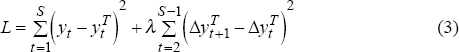
where λ is the smoothing weight on potential output growth and S is the sample size. Changing this weight affects how responsive potential output is to movements in actual output. As the smoothing factor approaches infinity, the loss function is minimised by penalising changes in potential growth, which is done by making potential output growth constant (i.e. a linear trend growth rate). As the smoothing factor approaches zero, the loss function is minimised by eliminating the difference between actual and potential output, which is done by making potential output equal to actual output. These features are captured in the left-hand panel in Figure 3, which shows estimates of the output gap for three smoothing factors, 6,000, 1,600 and 100, with a lower smoothing factor producing a ‘smaller’ estimate of the gap.
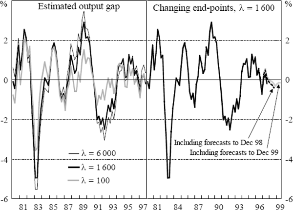
The advantage of the HP filter is that it renders the output gap stationary over a wide range of smoothing values (Hodrick and Prescott 1997) and it allows the trend to change over time. But it also has the distinct disadvantage that the selection of the smoothing weight is arbitrary, and that this matters to the estimate. For example, consider the estimate of the gap at December 1997 on the left-hand panel of Figure 3. For high smoothing, the estimate indicates output is above potential, but for moderate or low smoothing, the estimate suggests output is below potential. Indeed, for estimates using λ in the range 100 to 2,000, the gap is negative, but for values over this, the gap is positive. This method is not useful for identifying the absolute value of the output gap at a particular point in time.
Not only does the size of the gap vary with the smoothing weight, however, but so too do the relative scale and timing of peaks and troughs in output. For example, the left-side panel of Figure 3 shows that relatively high smoothing weights position output well above potential in 1989 compared with 1985, but a low smoothing weight reverses this relative scale. Similarly, a low smoothing weight marks 1991 as the time when output was most below potential while the higher smoothing weights mark 1992 as that point. In other words, information about the cycle changes with the smoothing weight.
If the smoothing parameter matters to the outcome, there has to be a clear method to select the smoothing parameter if the approach is to be useful. The smoothing parameter is conventionally set to 1,600 in empirical work. The ‘appropriate’ value depends on the relative size of the variances of the shocks to permanent and transitory components to output (Hodrick and Prescott 1997). Hodrick and Prescott (1997) chose the value of 1,600 for US GNP on the basis of their assessment of the relative size of shocks to that series. Guay and St Amant (1996) present Monte Carlo evidence, however, that a smoothing parameter of 1,600 is only appropriate under implausible joint assumptions about the relative importance of demand and supply shocks and about the persistence of cycles. There are other doubts about the accuracy of the HP filter in decomposing a time series into trend and cycle. For example, there is evidence that the accuracy of the decomposition varies over different data-generating processes and different data sets (King and Rebelo 1993; Harvey and Jaeger 1993).
A problem common to most estimates of potential output is that they can change as new data observations come to hand (which is separate to the issue of the estimate changing as data are revised). This also happens with the HP filter since it contains leads and lags of output in the loss function. It is only a symmetric two-sided filter at the middle of the sample, with end-points having more leverage. Using a sample of 128 observations, for example, St Amant and van Norden (1997) show that observations at the centre of the sample receive at most a six per cent weight while the last observation accounts for 20 per cent of the weight. The end-point problem implies that estimates of the gap at the end of the sample may be subject to substantial revision as new data come to hand, the period which is of most interest to policy-makers. This is illustrated in the right-side panel of Figure 3, where the sample is progressively extended using consensus forecasts of GDP for 1998 and 1999, with output growth projected to decelerate to about 3 per cent by the end of 1998 and then pick up to 3½ per cent by the end of 1999.[2] As the sample period is extended using this information, end-points are revised substantially, although (at least for the forecasts here) not more than when the smoothing parameter is changed. The size of the revision also depends on the cycle: the revision to the gap is larger at turning points than when the economy is at potential.
2.3 Multivariate Hodrick-Prescott Method
Linear detrending and the HP filter are statistical tools which do not use economic or structural information. There are economic relationships (the Phillips curve and Okun's Law) and economic indicators (capacity utilisation), however, which also contain information about the supply side of the economy and the stage of the business cycle. Accordingly, Laxton and Tetlow (1992) proposed an extension to the HP filter which incorporates such economic information. Potential output, for example, can be defined as the series which minimises the loss function:

where ε is a residual from a regression, the subscripts π, u and cu indicate a Phillips curve equation, Okun's Law equation and capacity utilisation equation respectively, and μ, β and ψ are possibly time-varying weights. The residuals are from the following equations:


Equation (5) is a Phillips curve, stating that inflation will be above expectations when output is above the (non-accelerating inflation) level of potential output. Equation (6) draws on Okun's Law, with the unemployment rate below the non-accelerating inflation rate of unemployment (NAIRU) when output is above potential. Equation (7) draws on a partial indicator of supply capacity, stating that capacity utilisation is above trend when output is above potential (Conway and Hunt 1997). These relationships, the data for which are shown in Figure 4, contain information about the output gap. The multivariate filter in Equation (4) sets potential output to minimise a weighted average of deviations of output from potential, changes in the potential rate of growth and errors in the three conditioning structural relationships. By conditioning the HP filter estimate of the output gap on this information, a more precise estimate of potential output, and hence the output gap, should be obtained.
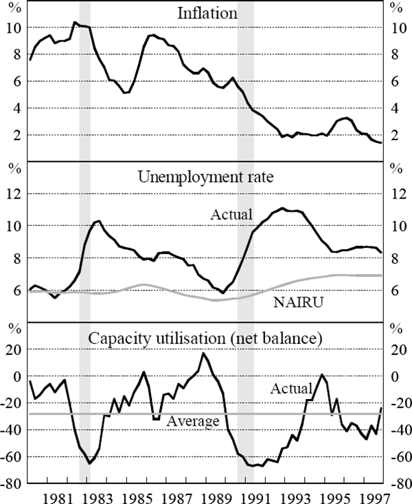
Note: Recessions, defined as two or more quarters of successive contraction in output, are shown as the shaded area.
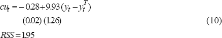
To proceed with this technique, Equations (5), (6) and (7) need to be specified. To obtain initial values for these equations, potential output is determined by the univariate HP filter value for λ = 1,600. To specify the Phillips curve in Equation (5), it is necessary to specify the expectations formation process. As a first approximation, it is assumed that expected inflation depends on lags of past consumer and imported price inflation (Debelle and Stevens 1995):
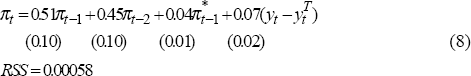
where π and π* are quarterly underlying inflation and import price inflation, the coefficients on the various inflation terms sum to one (a restriction which is not rejected by the data), RSS is the sum of squared residuals, and standard errors are shown in parentheses. In terms of using this equation to help identify potential output, this result suggests that current inflation contains information about the current gap.
To estimate Equation (6), the NAIRU is assumed to be the series estimated by Debelle and Vickery (1997), shown in the middle panel of Figure 4. Equation (6) is:
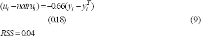
As expected, unemployment falls when current demand in the economy is strong relative to potential.
The capacity utilisation equation is estimated using the ACCI-Westpac survey measure of capacity utilisation for manufacturing firms, shown in the bottom panel of Figure 4.[3] The profile of capacity utilisation matches the profile of the recessions. There are a number of problems associated with using survey data as an indication of supply and demand imbalances, including whether firms clearly distinguish between labour and capital constraints, whether firms have a uniform definition of capacity and whether what they define to be ‘normal’ varies over the cycle. Moreover, when surveys are restricted to a particular sector, as is the case with the ACCI-Westpac measure, it is unclear how representative their responses are of the broader economy. For example, spare capacity widened during 1995 due to particular problems in the manufacturing sector.
The estimated equation for capacity utilisation is:
This suggests that current capacity utilisation contains information about the current state of the output gap.
Using these specifications for the Phillips curve, Okun's Law and capacity utilisation equations, the loss function in Equation (4) can be minimised to solve for potential output. The following iterative procedure is used to estimate potential output. As a first step, the conditioning equations are estimated using the univariate HP filter – Equations (8), (9) and (10) above – and the residuals are used to minimise the loss function in Equation (4) and solve for potential output. The output gap is computed and the coefficient on the output gap in the structural equations is re-estimated.[4] The loss function is minimised with these new residuals, and the coefficient on the output gap in the structural equations is recomputed. This procedure, similar to that outlined in Conway and Hunt (1997), is continued until the changes in the output gap coefficients satisfy a convergence criterion.
The issue of the weighting of the various components in the loss function also needs to be resolved. As is apparent from comparing the sum of squared residuals (RSS) for the three conditioning structural equations above, the residuals from the capacity utilisation equation are considerably larger than for the Phillips curve and Okun's Law equations. If the residuals are assigned equal weights in the loss function, then the loss function is essentially minimised by setting the gap to minimise the residual in the capacity utilisation equation (and, indeed, including a gap term calculated this way substantially reduces the residual sum of squares in the capacity utilisation equation). Similarly, the sum of squared deviations of output from trend is larger than for the Phillips curve and Okun's Law equations, which implies that if the weight on the deviations of output from potential are also not weighted, the loss function puts all the weight on the univariate HP filter components, making the multivariate and univariate gap estimates almost identical.
Accordingly, at each stage in the iteration, the sum of squared residuals for each of the
conditioning equations is weighted by its size relative to the sum of squared residuals of
output less potential. For example, the weight on the inflation equation residuals,
μ, is equal to 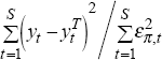 from the previous iteration (or, in the
case of the first iteration, the starting values). The larger is the sum of squared residuals in
the conditioning equation relative to the sum of squared output gaps, the smaller is its weight
in the loss function. The weight changes with each iteration. The top panel of Figure 5 shows
the gap estimated after convergence (which takes about 250 iterations).
from the previous iteration (or, in the
case of the first iteration, the starting values). The larger is the sum of squared residuals in
the conditioning equation relative to the sum of squared output gaps, the smaller is its weight
in the loss function. The weight changes with each iteration. The top panel of Figure 5 shows
the gap estimated after convergence (which takes about 250 iterations).
While the profiles of the gap estimated by the univariate and multivariate HP filters are very similar, such that they tend to move in the same direction, the size of the gap is very different for each of the filters. When the estimate of potential output is conditioned on additional economic information, the output gap is typically negative, indicating that actual has been below potential output for most of the past two decades except for the early and late 1980s.
This is explained by the unemployment equation, which, as shown in Figure 4, indicates that the unemployment rate has been above the estimated NAIRU for most of this period. The persistent wedge between the unemployment rate and the estimate of the NAIRU used here indicates that potential output has been higher than actual output.[5] The bottom panel of Figure 5 shows the estimate of the gap when the unemployment-output relation is excluded from the procedure. Since there is not a persistent wedge in the Phillips curve and capacity utilisation equation in the way that they have been estimated, potential output in this case is not estimated to have been systematically above actual output. The restricted set of conditioning information indicates that output was further below potential than indicated by the univariate HP filter in the early 1990s and in 1997, consistent with the weakness in capacity utilisation and declining inflation at these times.
The upshot of this experiment is that judgment matters. The estimate of the gap depends on the conditioning relationships, how those relationships are defined, and how the information is weighted in the loss function. When the output gap is conditioned on information which contains a constant wedge between the unemployment rate and the NAIRU, there is a substantial negative output gap. Once this wedge is removed, the gap narrows considerably. The way the conditioning relationships are modelled is of critical importance to the estimate of the output gap. Moreover, instead of assuming that the weights for the conditioning variables are constant over the sample period, the modeller can change the weights to reflect his or her assessment of the relative importance of the conditioning information at different times. Similarly, estimates of the gap towards the end of the sample will change when forecasts are included.
2.4 Unobservable Components Method
Given that potential output and the gap are unknown, it makes sense to use statistical techniques which can decompose a time series into unobservable components, such as that set out by Watson (1986). For example, output (y) can be decomposed into a permanent (yp) and a transitory component (z):

where the permanent and transitory components correspond to the potential and gap terms in Equation (1). Permanent, or potential, output is assumed to follow a random walk with drift:

where μy is a drift term and  . Since the
estimation is from 1980 to 1997, and hence excludes the structural break in growth in the 1970s,
the drift term is assumed to be constant. The output gap is assumed to follow an AR(2) process:
. Since the
estimation is from 1980 to 1997, and hence excludes the structural break in growth in the 1970s,
the drift term is assumed to be constant. The output gap is assumed to follow an AR(2) process:

where  and
the stationarity conditions hold.
and
the stationarity conditions hold.
This can be written in state-space form (Kuttner 1994; Gerlach and Smets 1997). Using the terminology of Harvey (1981), the vector of observed variables – a single variable, output, in the example described above – is denoted as Y, while the vector of unobserved state variables – the trend growth rate, permanent output and the output gap in this case – is denoted by α. The evolution of the observed variables is described in the measurement equation as a function of the unobserved state variables:

where Z is a matrix of coefficients, d is a matrix of exogenous variables and ε is a vector of white-noise errors weighted by S. The time series processes for the unobserved state variables are set out in the transition equation:

where T is a matrix of coefficients, c is a matrix of exogenous variables and ε is a vector of white-noise errors weighted by η. Appendix A sets out the model more explicitly.
Estimates of the parameters of the model and the unobserved state variables can be obtained by maximising the likelihood function:
using the Kalman filter, where N is the number of observed variables, S is the sample size, v is the prediction error matrix and F is the mean square error matrix for the prediction errors. The initial values for the estimation were obtained using the HP filter with λ = 1,600 and are shown in the first column of Table 2. The final estimated coefficients from this model are shown in the second column of Table 2, and the top panel of Figure 6 shows the estimate of the output gap.
| Initial estimates (HP model, λ = 1,600) |
UC model of output |
UC model of output and inflation |
|
|---|---|---|---|
| μy | 0.0078 (0.00001) |
0.0077 | 0.0077 |
| ϕ1 | 1.15 (0.11) |
1.52 | 1.26 |
| ϕ2 | −0.35 (0.11) |
−0.61 | −0.42 |
| μπ | −0.0001 (0.0004) |
– | 0.0000 |
| δ1 | 0.50 (0.10) |
– | 0.96 |
| δ2 | 0.46 (0.10) |
– | 0.00 |
| β | 0.07 (0.02) |
– | 0.05 |
| Standard error (εy) | 0.0014 | 0.0060 | 0.0030 |
| Standard error (εz) | 0.0080 | 0.0051 | 0.0043 |
| Standard error (επ) | 0.0029 | – | 0.0013 |
|
Notes: Standard errors in brackets. |
|||
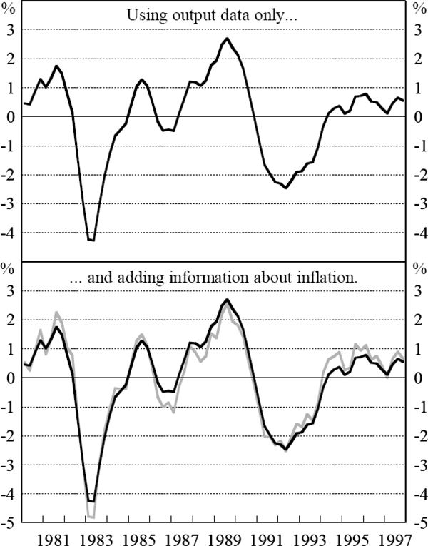
This estimate is a univariate decomposition of output. Kuttner (1994) has extended the model to include information about the output gap contained in the Phillips curve, assuming that inflation is below the expected rate of inflation when output is below potential (a negative gap). Gerlach and Smets (1997) have used this approach to estimate output gaps for the G7 economies. Following this, Equation (17) sets out an equation for the Phillips curve assuming that inflation expectations depend on past values of inflation of consumer price and imported goods and services:

where the error is also white noise. A constant term is included for generality but is expected to be zero. Appendix A also sets out the equations for the general state-space form when inflation is modelled this way and is included in the model.
Initial parameter estimates were obtained by estimating Equation (17) using the HP estimate of the output gap, and these are also presented in the first column of Table 2. The unobservable components estimate of the output gap which conditions on both the output and inflation data is shown in the bottom panel of Figure 6, and the coefficient estimates are set out in the third column of Table 2. The profile of the output gap is very similar when information about inflation is used, but the size of the gap varies at times. For example, demand conditions appear relatively weaker in the late 1980s when inflation is included, presumably because the Accord dampened wage rises, which are an important driving force in the inflation process. Similarly, demand conditions appear a little stronger in 1994 than suggested by just looking at output, presumably because inflation accelerated strongly at this time.
2.5 Production Function Method
An alternative, ‘structural’, approach is to estimate the output gap as actual output less potential output calculated on the basis of an aggregate production function (see, for example, Laxton and Tetlow 1992; OECD 1994; Giorno et al. 1995; De Masi 1997; Fisher et al. 1997). For example, suppose that output can be characterised as a Cobb-Douglas production function:

where y is output, tfp is total factor productivity, l is effective labour and k is the capital stock, α is the labour share of income, and variables are in logarithms. If the inputs are equilibrium values, then the production function provides an estimate of potential output and hence the output gap.
This is typically made operational in the following way. First, using historical values of the labour share of income (α = 0.57), total factor productivity is estimated as output less the weighted sum of effective labour and physical capital inputs:

Output is GDP(A). Effective labour is defined as full-time-equivalent employment multiplied by the ratio of the trend participation rate to the actual participation rate. Full-time equivalent employment is used since this corrects for changes in ‘labour intensity’ associated with an increase in the share of part-time jobs. It is calculated as full-time employment plus 15/40 times part-time employment. Employment also changes over the cycle because of changes in the participation rate, and the effect of this is removed by multiplying full-time-equivalent employment by the ratio of trend to actual participation. The trend in the participation rate is estimated as a linear trend from 1980 to 1997. The estimate of capital is the published capital stock, interpolated to give a quarterly series. The top panel of Figure 7 plots the natural log of indices of output, labour and capital.
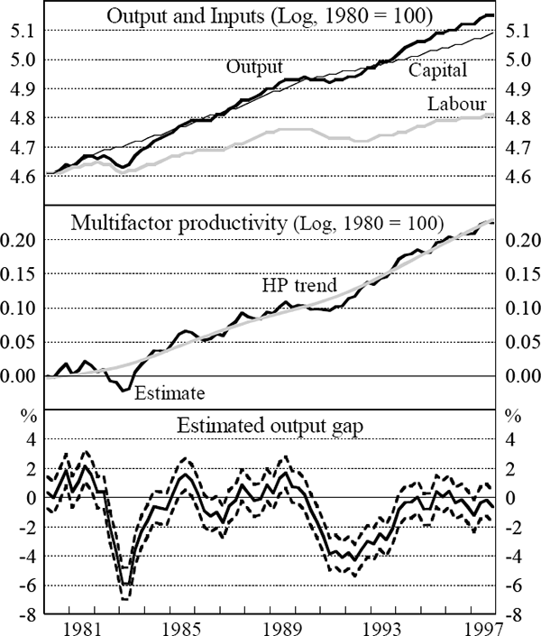
A trend is then fitted to the residual, total factor productivity, in order to obtain an estimate of trend productivity to be used in calculating potential output. There are many techniques to calculate a trend. Since productivity growth changes over time, a simple linear trend is inappropriate. An HP filter is used to estimate trend total factor productivity, and is shown in the second panel of Figure 7 with the estimate of total factor productivity from Equation (19). While use of the HP filter is arbitrary, it is no less so than alternative methods such as estimated or judgmental linear break-in-trend models. This estimate indicates that total factor productivity has been growing around 1.8 per cent a year since 1994.
Potential output can then be estimated as trend total factor productivity plus the weighted sum of full-employment effective labour and the capital stock. Full-employment labour is assumed to be that level of employment consistent with non-accelerating inflation, and we use Debelle and Vickery's (1997) estimate of the NAIRU for this calculation:

where lf is the labour force, nairu is the non-accelerating-inflation rate of unemployment, p is the participation rate, ftequiv is full-time equivalent employment, N is employment and a superscript T indicates a (linear) trend. The trend in the ratio of full-time-equivalent employment to total employment is used instead of the actual ratio in order to abstract from cyclical variation. The output gap is actual less potential output. The bottom panel of Figure 7 shows this estimate, together with a one standard error confidence band based on the standard error from the estimate of trend total factor productivity. These standard errors are one way to indicate the imprecision of estimates of the output gap. To the extent that there is uncertainty about the full-employment labour force and the capital stock (which is certainly the case), the ‘true’ standard error is larger (Fisher et al. 1997).
The production function approach has been criticised on a number of grounds – that the economic structure changes, often in a way that is not known, that the method still uses simple detrending procedures (such as the HP filter) which have an important bearing on the gap estimate, that a range of ad hoc assumptions are made about potential labour and capital, and that the data on the capital stock are of poor quality (Laxton and Tetlow 1992; Conway and Hunt 1997). These criticisms are valid but most of them also apply to other methods, and the production function approach has a strong intuitive appeal and is widely used (Giorno et al. 1995; De Masi 1997).
Footnotes
The working paper version was written in 1980 but was not published until 1997. [1]
The Consensus forecasts at March 1998 for year-on-year growth for the eight quarters in 1998 and 1999 are 4.1, 3.1, 2.8, 3.1, 3.1, 3.3, 3.4 and 3.5 per cent. [2]
This survey is reported as a net balance of respondents who think that they are working above their normal capacity. [3]
To make the estimation process simpler, the procedure maintains the original slope coefficients for all variables in the conditioning equations apart from the output gap. This assumes orthogonality between regressors. The equations were re-estimated with the final multivariate HP gap measure with only minimal change in the slope coefficients on the non-gap terms. [4]
The unemployment equation embodies the assumption that output is at potential when expected inflation equals actual inflation, rather than the assumption that output is at potential when inflation is steady. The measures of expected inflation used by Debelle and Vickery to estimate the NAIRU have been systematically above actual inflation, and this gives rise to the wedge between the unemployment rate and the NAIRU. Only when actual and expected inflation are equal, is the unemployment rate at the NAIRU. Other measures of expected inflation may yield different estimates of the NAIRU, and so this number is illustrative only. [5]