RDP 9704: Financial Aggregates as Conditioning Information for Australian Output and Inflation 4. The Single-equation Methodology
July 1997
- Download the Paper 139KB
The approach here is to examine whether lagged or contemporaneous values of the growth in financial aggregates adds explanatory power to intensively specified single-equation models of inflation and real output growth for Australia. We view a particular financial aggregate as having useful information value if it is statistically significant in either of these models. We employ the same financial aggregate measures as those used in the first section of this paper, and use this exercise as a robustness check of information content across empirical methods.
Our base model for real output growth originates from Gruen and Shuetrim (1994) whereas the model for inflation is a revised version of that used in de Brouwer and Ericsson (1995). The preferred specifications in these papers are the end result of extensive investigation into the determinants of real output growth and inflation over their respective samples and data sets. In this study our concern is not in finding the optimal models for real output growth and inflation; rather, we focus solely on examining whether information on financial aggregates helps predict movements in either real output growth or inflation using the single-equation models as the base case.
Before adding information on financial aggregates, we examine whether the specifications used in both studies were stable after extending the data sample to 1996:Q2. In their original specifications, the estimates for each model employ a shorter dataset. Gruen and Shuetrim (1994) and de Brouwer and Ericsson (1995) estimate their models over the data samples 1980:Q1 to 1993:Q4 and 1977:Q3 to 1993:Q3, respectively. A slightly altered version of the preferred specification from Gruen and Shuetrim (1994) appeared to remain adequate over our full sample 1980:Q3 to 1996:Q2.[11] In contrast, the preferred model in de Brouwer and Ericsson (1995) failed to hold up over the extended sample. Significant revisions in the data used by de Brouwer and Ericsson altered the fit of their preferred specification over their original sample 1977:Q3 to 1993:Q3.
4.1 Model of Real Output Growth
The Gruen and Shuetrim (1994) model is specified as follows,

where Δyt is Australian quarterly GDP growth, rt is the real
short-term interest rate,  is a measure of the growth in the agricultural
component of Australian output, yt-1 and wt-1
are lagged log-levels of Australian and foreign activity, and Δwt
is the contemporaneous quarterly growth rate in foreign activity. The foreign
activity variable is used to capture its anticipated positive effect on growth
in domestic activity. Gruen, Romalis and Chandra (1997) suggest that US GDP
is better than OECD GDP as a proxy for measuring the effect of foreign activity
on Australian output. In this paper, OECD GDP and US GDP are used to measure
foreign activity in alternative specifications of the output growth equation.
The inclusion of the lagged log-level terms is to capture a possible long-run
relationship between the levels of domestic and foreign
activity.[12]
The lags of real short-term interest rate are used to control for the effects
of domestic monetary policy and the mean of the coefficients on these terms
is expected to be negative. A detailed discussion of the data used in estimation
of this equation is in Appendix A.
is a measure of the growth in the agricultural
component of Australian output, yt-1 and wt-1
are lagged log-levels of Australian and foreign activity, and Δwt
is the contemporaneous quarterly growth rate in foreign activity. The foreign
activity variable is used to capture its anticipated positive effect on growth
in domestic activity. Gruen, Romalis and Chandra (1997) suggest that US GDP
is better than OECD GDP as a proxy for measuring the effect of foreign activity
on Australian output. In this paper, OECD GDP and US GDP are used to measure
foreign activity in alternative specifications of the output growth equation.
The inclusion of the lagged log-level terms is to capture a possible long-run
relationship between the levels of domestic and foreign
activity.[12]
The lags of real short-term interest rate are used to control for the effects
of domestic monetary policy and the mean of the coefficients on these terms
is expected to be negative. A detailed discussion of the data used in estimation
of this equation is in Appendix A.
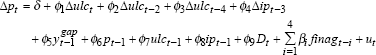
4.2 Model of Inflation
Given the revisions to the data used in de Brouwer and Ericsson (1995), we search for a comparable model of inflation, using their general model of inflation and a general to specific approach to arrive at the following parsimonious specification,[13]
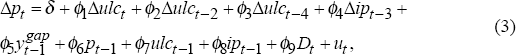
where p is the underlying CPI, ulc is unit labour costs, ip is import prices, ygap is the output gap term and D is a dummy variable included for an increase in indirect taxes in December 1978. Positive movements in the growth rate of both unit labour costs and import prices are expected to increase inflation. The inclusion of lagged level terms is to capture long-run relationships between inflation, unit labour costs, and import prices. The coefficients on all the lagged log-level terms are expected to be positive except for the lagged log-level of the dependent variable. A detailed discussion of the data used in estimation of this equation is in Appendix A.
4.3 Empirical Methods
We examine whether past information on financial aggregates is useful for explaining current movements in real output growth or inflation by including four lags of financial aggregate growth in both equations.[14] For the real output growth equation, the appropriate transformation of the financial aggregate is a real growth measure, whereas for the inflation equation, nominal aggregate growth is the relevant measure. We estimate each equation by OLS and then examine F-tests of two restrictions – first, that the coefficients on the financial aggregate terms sum to zero, and second, whether each of the four coefficients for the financial aggregate measure should be restricted to zero. The first restriction implies a prior belief that the net effect of financial aggregate growth should be positive. The second restriction suggests whether the lags of the financial aggregate growth rates are at all related to the policy variables. We employ these tests for the full-sample estimation.
Data for real GDP and CPI are released on a quarterly basis whereas financial aggregate data are released on a monthly basis, and available prior to the release of real GDP and CPI data. Consequently, information available on financial aggregates in the same quarter may be useful for predicting current movements in the policy variables. If there is significant contemporaneous correlation between financial aggregates and growth in the variable, then the first two months of data on the particular financial aggregate could be exploited to predict movement in growth of the relevant variable. To examine this issue, we investigate whether contemporaneous growth in the financial aggregates is significant in estimations of the real output growth and inflation equations.[15] Due to simultaneity problems between the contemporaneous growth in financial aggregates and current movement in real output growth and inflation, we estimate these models by the instrumental variables estimation technique. The first lag of the growth in the relevant financial aggregate is used as one of the instruments for the contemporaneous growth in the financial aggregate in these regressions. We then test the exclusion of the contemporaneous growth in the financial aggregate in each respective equation.
Our significance criteria for a useful information variable requires that the relevant restriction be rejected at the 5 per cent significance level. The results are presented in Tables 3 through 6. Using our criteria, we find in no case, either lagged or contemporaneously, that nominal growth in any of the financial aggregates has useful information content for the model of inflation. For output, we find significant results for both lagged and contemporaneous real credit growth as predictors for real output growth in the regressions using OECD output.[16] However, when US GDP is the foreign output proxy, there is no evidence that any of the financial aggregates provide explanatory power to the real output growth regression.
| Variables |
Original model | Model with M3 | Model with BM | Model with M1 | Model with CRED | Model with CURR |
|---|---|---|---|---|---|---|
| Constant | −1.67** (−3.04) | −1.67** (−2.94) | −1.83 (−3.02) | −1.50* (−2.60) | −3.19** (−4.88) | −1.69** (−2.92) |
| Real cash rate(b) | −0.0004 {0.00}** | −0.0004 {0.00}** | −0.0004 {0.00}** | −0.0004 {0.02}** | −0.0006 {0.00}** | −0.0004 {0.00}** |
| Lagged Australian GDP log level | −0.21** (−2.93) | −0.21** (−2.84) | −0.23** (−2.91) | −0.19* (−2.60) | −0.40** (−4.77) | −0.21** (−2.82) |
| Lagged OECD GDP log level | 0.26** (3.11) | 0.26** (3.00) | 0.28** (3.09) | 0.23* (2.61) | 0.49** (4.95) | 0.26** (2.99) |
| OECD GDP growth | 1.05** (4.85) | 1.02** (4.13) | 1.03** (4.05) | 0.93** (3.61) | 0.79** (3.48) | 1.11** (4.74) |
| Farm GDP growth(b) | 0.017 {0.09} | 0.016 {0.11} | 0.016 {0.11} | 0.014 {0.22} | 0.023 {0.08} | 0.016 {0.15} |
| Growth in aggregate [1] | −0.001 (−0.01) | −0.038 (−0.30) | 0.021 (0.35) | 0.043 (0.38) | −0.074 (−0.76) | |
| Growth in aggregate [2] | 0.060 (0.60) | 0.140 (1.23) | 0.090 (1.81) | 0.078 (0.65) | 0.058 (0.61) | |
| Growth in aggregate [3] | 0.005 (0.05) | 0.070 (0.60) | 0.040 (0.72) | 0.090 (0.76) | 0.068 (0.73) | |
| Growth in aggregate [4] | −0.014 (−0.14) | 0.020 (0.18) | −0.030 (−0.54) | 0.190 (1.55) | −0.078 (−0.75) | |
| Exclusion of lags of financial aggregate | {0.98} |
{0.70} |
{0.41} |
{0.013}* |
{0.76} |
|
| Test of sum of lags of financial aggregate | {0.75} |
{0.37} |
{0.22} |
{0.00}** |
{0.87} |
|
| Adjusted R2 | 0.41 | 0.37 | 0.39 | 0.41 | 0.50 | 0.38 |
| LM test for 1st order autocorrelation | 0.31 {0.58} | 0.41 {0.52} | 0.55 {0.46} | 0.71 {0.40} | 0.31 {0.58} | 0.48 {0.49} |
| Notes: (a) The models are estimated by OLS. Numbers in square brackets [
] are lags. Numbers in parentheses ( ) are t-statistics. Numbers in braces
{} are p-values. Items marked with *(**) are significantly different from
zero at the 5%(1%) level. All variables in log levels (except for real
interest rate). (b) The mean coefficient is reported for the real cash rate and farm growth. The p-values for the real interest rate and farm growth are derived from F-tests of the joint significance of the lags. |
||||||

| Variables |
Original model | Model with M3 | Model with BM | Model with M1 | Model with CRED | Model with CURR |
|---|---|---|---|---|---|---|
| Constant | −1.25** (−5.04) | −1.23** (−4.69) | −1.21 (−4.64) | −1.17** (−4.16) | −1.41** (−5.26) | −1.28** (−4.77) |
| Real cash rate(b) | −0.0004 {0.00}** | −0.0004 {0.00}** | −0.0004 {0.00}** | −0.0004 {0.02}** | −0.0005 {0.00}** | −0.0004 {0.00}** |
| Lagged Australian GDP log level | −0.28** (−4.98) | −0.27** (−4.65) | −0.27** (−4.58) | −0.26** (−4.19) | −0.31** (−5.17) | −0.28** (−4.71) |
| Lagged US GDP log level | 0.33** (5.19) | 0.33** (4.80) | 0.32** (4.76) | 0.31** (4.15) | 0.38** (5.42) | 0.34** (4.89) |
| US GDP growth | 0.35** (2.92) | 0.34** (2.71) | 0.37** (2.82) | 0.31* (2.38) | 0.33** (2.71) | 0.35** (2.77) |
| Farm GDP growth(b) | 0.018 {0.03}* | 0.018 {0.04}* | 0.018 {0.04}* | 0.014 {0.16} | 0.018 {0.024}* | 0.019 {0.04}* |
| Growth in aggregate [1] | −0.002 (−0.02) | −0.038 (−0.35) | 0.033 (0.61) | −0.120 (−1.09) | −0.069 (−0.76) | |
| Growth in aggregate [2] | 0.050 (0.54) | 0.080 (0.79) | 0.053 (1.06) | −0.090 (−0.75) | −0.006 (−0.07) | |
| Growth in aggregate [3] | 0.019 (−0.20) | −0.010 (−0.11) | 0.007 (0.15) | 0.100 (0.87) | 0.075 (0.88) | |
| Growth in aggregate [4] | −0.004 (−0.04) | −0.020 (−0.19) | −0.060 (−1.10) | 0.190 (1.66) | −0.023 (−0.24) | |
| Exclusion of lags of financial aggregate | {0.99} |
{0.95} |
{0.70} |
{0.22} |
{0.86} |
|
| Test of sum of lags of financial aggregate | {0.86} |
{0.94} |
{0.71} |
{0.28} |
{0.88} |
|
| Adjusted R2 | 0.50 | 0.46 | 0.46 | 0.48 | 0.52 | 0.47 |
| LM test for 1st order autocorrelation | 0.68 {0.41} | 0.92 {0.34} | 0.61 {0.44} | 1.76 {0.19} | 0.86 {0.35} | 0.89 {0.35} |
| Notes: (a) The models are estimated by OLS. Numbers in square brackets [
] are lags. Numbers in parentheses ( ) are t-statistics. Numbers in braces
{} are p-values. Items marked with *(**) are significantly different from
zero at the 5%(1%) level. All variables in log levels (except for real
interest rate). (b) The mean coefficient is reported for the real cash rate and farm growth. The p-values for the real interest rate and farm growth are derived from F-tests of the joint significance of the lags. |
||||||

| Variables |
Original model |
Model with M3 |
Model with BM |
Model with M1 |
Model with CRED |
Model with CURR |
|---|---|---|---|---|---|---|
| Constant | −1.67** (−3.04) | −1.61** (−2.68) | −1.61 (−1.88) | −1.02 (−0.27) | −2.44** (−3.92) | −2.25 (−1.78) |
| Real cash rate(b) | −0.0004 {0.00}** | −0.0004 {0.00}** | −0.0005 {0.52} | −0.0004 {0.02}* | −0.0003 {0.00}** | −0.0005 {0.03}* |
| Lagged Australian GDP log level | −0.21** (−2.93) | −0.20* (−2.63) | −0.20 (−1.70) | −0.13 (−0.31) | −0.31** (−3.82) | −0.28 (−1.73) |
| Lagged OECD GDP log level | 0.26** (3.11) | 0.25** (2.71) | 0.25* (2.04) | 0.16 (0.26) |
0.37** (3.98) | 0.35 (1.81) |
| OECD GDP growth | 1.05** (4.85) | 1.00** (3.29) | 1.14 (1.43) | 0.84 (0.66) |
0.71** (2.78) | 1.21** (3.15) |
| Farm GDP growth(b) | 0.017 {0.09} | 0.017 {0.09} | 0.016 {0.13} | 0.012 {0.29} | 0.017 {0.06} | 0.018 {0.15} |
| Growth in aggregate | 0.05 (0.22) |
−0.14 (−0.11) | 0.26 (0.17) |
0.30* (2.31) | −0.35 (−0.54) | |
| Exclusion of financial aggregate | {0.82} |
{0.91} |
{0.86} |
{0.02}* |
{0.59} |
|
| Adjusted R2 | 0.41 |
0.41 |
0.31 |
0.19 |
0.46 |
0.17 |
| LM test for 1st order autocorrelation | 0.31 {0.58} |
0.34 {0.56} |
8.75 {0.00}** | 17.18 {0.00}** | 1.10 {0.30} |
15.04 {0.00}** |
| Notes: (a) The models are estimated by instrumental variables. Numbers in
square brackets [ ] are lags. Numbers in parentheses ( ) are t-statistics.
Numbers in braces {} are p-values. Items marked with *(**) are significantly
different from zero at the 5%(1%) level. All variables in log levels (except
for real interest rate). (b) The mean coefficient is reported for the real cash rate and farm growth. The p-values for the real interest rate and farm growth are derived from F-tests of the joint significance of the lags. |
||||||

| Variables |
Original model |
Model with M3 |
Model with BM |
Model with M1 |
Model with CRED |
Model with CURR |
|---|---|---|---|---|---|---|
| Constant | −1.67** (−3.04) | −1.22** (−4.00) | −1.32** (−3.33) | −0.72 (−0.40) | −1.27** (−4.00) | −1.73* (−2.02) |
| Real cash rate(b) | −0.0004 {0.00}** | −0.0004 {0.00}** | −0.0005 {0.20} | −0.0004 {0.04}* | −0.0004 {0.00}** | −0.0005 {0.02}* |
| Lagged Australian GDP log level | −0.21** (−2.93) | −0.27** (−4.01) | −0.29** (−3.33) | −0.17 (−0.43) | −0.28** (−3.94) | −0.39 (−1.99) |
| Lagged US GDP log level | 0.26** (3.11) | 0.33** (4.00) | 0.35* (3.24) | 0.19 (0.36) |
0.34** (4.11) | 0.45* (2.06) |
| US GDP growth | 1.05** (4.85) | 0.34* (2.50) | 0.39 (1.85) |
0.33 (1.85) |
0.35** (2.89) | 0.27** (3.15) |
| Farm GDP growth(b) | 0.017 {0.09} | 0.018 {0.03} | 0.018 {0.05} | 0.012 {0.20} | 0.018 {0.03} | 0.019 {0.08} |
| Growth in aggregate | 0.035 (0.17) | −0.16 (−0.24) | 0.33 (0.30) |
−0.01 (−0.13) | −0.39 (−0.60) | |
| Exclusion of financial aggregate | {0.87} |
{0.81} |
{0.77} |
{0.90} |
{0.55} |
|
| Adjusted R2 | 0.41 | 0.49 | 0.41 | 0.07 | 0.46 | 0.27 |
| LM test for 1st order autocorrelation | 0.31 {0.58} |
0.50 {0.48} |
11.79 {0.00}** | 29.54 {0.00}** | 0.87 {0.35} |
20.96 {0.00}** |
| Notes: (a) The models are estimated by instrumental variables. Numbers in
square brackets [ ] are lags. Numbers in parentheses ( ) are t-statistics.
Numbers in braces {} are p-values. Items marked with *(**) are significantly
different from zero at the 5%(1%) level. All variables in log levels (except
for real interest rate). (b) The mean coefficient is reported for the real cash rate and farm growth. The p-values for the real interest rate and farm growth are derived from F-tests of the joint significance of the lags. |
||||||

| Variables |
Original model | Model with M3 | Model with BM | Model with M1 | Model with CRED | Model with CURR |
|---|---|---|---|---|---|---|
| Constant | −0.005 (−0.63) | −0.003 (−0.38) | −0.002 (−0.23) | −0.0008 (−3.08) | −0.003 (−0.34) | −0.004 (−0.45) |
| Growth in ULC [0] | 0.063** (3.65) | −0.060** (3.35) | 0.062** (3.31) | 0.056** (2.98) | 0.060** (3.59) | 0.062** (3.35) |
| Growth in ULC [2] | 0.052** (2.99) | 0.050** (2.67) | 0.051** (2.73) | 0.051** (2.74) | 0.056** (3.10) | 0.053** (2.87) |
| Growth in ULC [4] | 0.035* (2.15) | 0.036* (2.20) | 0.036* (2.12) | 0.035 (1.99) | 0.023 (1.29) | 0.035* (2.07) |
| Growth in import prices [3] | 0.036** (3.70) | 0.040** (3.72) | 0.040** (3.59) | 0.035** (3.22) | 0.030** (3.22) | 0.040** (3.35) |
| Output gap [1] | 0.073** (6.06) | 0.093** (5.23) | 0.079** (3.78) | 0.072** (5.65) | 0.055 (3.01} | 0.073** (5.80) |
| Lagged CPI log level | −0.073** (−7.65) | −0.075** (−7.57) | −0.073** (−6.90) | −0.069** (−6.18) | −0.067** (−6.86) | −0.073** (−6.89) |
| Lagged ULC log level | 0.042** (4.21) | 0.042** (4.18) | 0.041** (3.91) | 0.036** (2.89) | 0.039** (3.93) | 0.040** (3.98) |
| Lagged import price log level | 0.034** (10.25) | 0.036** (9.72) | 0.034** (8.49) | 0.035** (9.29) | 0.030** (6.21) | 0.030** (8.75) |
| Dummy | −0.005* (−2.03) | −0.005 (−1.81) | −0.005* (−2.01) | −0.005* (−2.09) | −0.005* (−2.09) | −0.005 (−1.98) |
| Growth in aggregate [1] | −0.059* (−2.19) | −0.007 (−0.22) | −0.013 (−0.79) | 0.002 (0.07) | 0.017 (0.55) | |
| Growth in aggregate [2] | 0.004 (0.12) | −0.019 (−0.53) | −0.006 (−0.36) | −0.060 (−1.47) | −0.020 (−0.70) | |
| Growth in aggregate [3] | 0.021 (0.21) | 0.015 (0.39) | −0.009 (−0.52) | 0.050 (1.31) | −0.005 (−0.15) | |
| Growth in aggregate [4] | −0.007 (−0.23) | −0.009 (−0.26) | 0.003 (0.17) | 0.050 (1.47) | 0.002 (0.06) | |
| Exclusion of lags of financial aggregate | {0.27} |
{0.97} |
{0.91} |
{0.17} |
{0.94} |
|
| Test of sum of lags of financial aggregate | {0.11} |
{0.75} |
{0.45} |
{0.24} |
{0.87} |
|
| Adjusted R2 | 0.90 | 0.90 | 0.89 | 0.89 | 0.90 | 0.89 |
| LM test for 1st order autocorrelation | 0.37 {0.55} | 0.92 {0.34} | 0.35 {0.55} | 0.30 {0.58} | 0.34 {0.56} | 0.57 {0.45} |
| Note: (a) The models are estimated by OLS. Numbers in square brackets [ ] are lags. Numbers in parentheses ( ) are t-statistics. Numbers in braces {} are p-values. Individual coefficients marked with *(**) are significantly different from zero at the 5%(1%) level. All variables in log levels. | ||||||
| Variables |
Original model | Model with M3 | Model with BM | Model with M1 | Model with CRED | Model with CURR |
|---|---|---|---|---|---|---|
| Constant | −0.005 (−0.63) | 0.0009 (0.08) | −0.004 (−0.28) | −0.012 (−3.08) | −0.005 (−0.63) | −0.009 (−0.63) |
| Growth in ULC [0] | 0.063** (3.65) | 0.046 (3.35) | 0.062** (2.61) | 0.064** (2.72) | 0.060** (3.61) | 0.063** (3.01) |
| Growth in ULC [2] | 0.052** (2.99) | 0.051* (2.37) | 0.052** (2.93) | 0.072 (1.60) | 0.053** (2.98) | 0.056* (2.39) |
| Growth in ULC [4] | 0.035* (2.15) | 0.040 (1.97) | 0.036* (2.05) | 0.030 (1.28) | 0.036 (2.09) | 0.032 (1.54) |
| Growth in import prices [3] | 0.036** (3.70) | 0.021 (1.38) | 0.040** (3.60) | 0.056 (1.37) | 0.040** (3.66) | 0.050 (1.37) |
| Output gap [1] | 0.073** (6.06) | 0.098** (4.57) | 0.075** (3.08) | 0.110 (1.56) | 0.072** (4.74} | 0.081** (3.14) |
| Lagged CPI log level | −0.073** (−7.65) | −0.076** (−6.38) | −0.073** (−7.50) | −0.082** (−3.72) | −0.073** (−7.47) | −0.064* (−2.40) |
| Lagged ULC log level | 0.042** (4.21) | 0.038** (3.05) | 0.041** (3.52) | 0.059 (1.62) | 0.042** (4.10) | 0.040** (2.56) |
| Lagged import price log level | 0.034** (10.25) | 0.040** (7.33) | 0.034** (7.33) | 0.027 (1.81) | 0.030** (6.99) | 0.030* (2.00) |
| Dummy | −0.005* (−2.03) | −0.007* (−2.13) | −0.005* (−1.86) | −0.004 (−0.93) | −0.005* (−2.00) | −0.004 (−1.20) |
| Growth in aggregate [0] | −0.130 (−1.62) | −0.010 (−0.10) | 0.110 (0.51) | 0.004 (0.12) | 0.130 (0.39) | |
| Exclusion of lags of financial aggregate | {0.11} |
{0.92} |
{0.61} |
{0.91} |
{0.70} |
|
| Adjusted R2 | 0.90 | 0.84 | 0.89 | 0.81 | 0.90 | 0.85 |
| LM test for 1st order autocorrelation | 0.37 {0.55} | −29.13 {n.a.} | −8.48 {n.a.} | 29.3 {0.00}** | 0.34 {0.56} | −1386.9 {0.70} |
| Note: (a) The models are estimated by OLS. Numbers in square brackets [ ] are lags. Numbers in parentheses ( ) are t-statistics. Numbers in braces {} are p-values. Items marked with *(**) are significantly different from zero at the 5%(1%) level. All variables in log levels. | ||||||
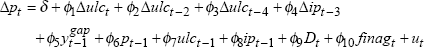
Table 3a presents the results for tests of the significance of lags in the growth rate of the financial aggregates in the real output growth equation using the OECD GDP variable. We focus on the properties of the specification that contains real credit growth. Both restrictions on the lags of the coefficients are rejected at the 5 per cent significance level, and the adjusted R-squared for the regression increases from 0.41 in the base regression to 0.50. Also, the coefficients of most regressors in the base specification remain statistically significant after the addition of the credit variables. Table 4a highlights the fact that the addition of contemporaneous credit growth has comparable effects to those mentioned above.[17]
In Tables 3b and 4b, we present results for the estimations of the real output growth equation using US GDP as the foreign output measure. We find that there is no instance in which any of the financial aggregates has a statistically significant impact on real output growth.
Notably, the base regression using US GDP (without lags of a real aggregate growth rate) has comparable explanatory power to the regression containing both OECD output and four lags of real credit growth. One way to interpret this finding is that US GDP conveys the information that both OECD GDP and real credit growth provide for the alternative real output growth specification. Another interpretation is that the result suggesting that real credit growth helps explain real output growth is not robust. Failure of the real credit results to be robust to an alternative measure of agricultural output, and to the exclusion of the real interest rate, support the latter interpretation.[18]
Footnotes
There was a large outlier in the OECD output measure in 1980:Q2 that made the statistical fit questionable over the entire sample. We dropped the first two observations to establish a satisfactory regression. [11]
Refer to Gruen and Shuetrim (1994) for a more detailed explanation of their model specification. [12]
The general model that we use is the same as Equation (11) in de Brouwer and Ericsson (1995) minus the seasonal dummies. [13]
We investigated whether the lag length on the aggregate has any impact on the inferences. We found no notable changes in our inferences from changes in the lag length on the aggregates. Results are available upon request from the authors. [14]
As above, we employ real aggregate measures in the real output growth equation and nominal aggregate measures in the inflation equation. [15]
The results for credit do not hold up if the farm output variable is replaced with the Southern Oscillation Index, the original proxy measure for Australian agricultural output used in Gruen and Shuetrim (1994). [16]
To examine the dynamics of the model with real credit growth, we estimate the impact of a temporary 1 per cent increase in the growth rate of real credit on the level of real output from the model using OECD GDP. The shock to real credit growth is distributed evenly over the first four quarters of the simulation. We find that after six quarters the cumulative impact on the level of real output is approximately 0.6 of a per cent. Results of this exercise are available upon request. [17]
One criticism of the real output growth equation for testing the information from monetary aggregate growth is that the real interest rate may capture much of the potential information that is available for real output growth from the financial sector of the economy. We estimate the real output growth equation (using both OECD and US output as the world output measure) without the real interest rate, and find that no financial aggregate has significant explanatory power for real output growth in this specification. [18]