RDP 9608: Modelling the Australian Exchange Rate, Long Bond Yield and Inflationary Expectations 3. A Behavioural Model of the Australian Real Exchange Rate
November 1996
- Download the Paper 171KB
3.1 What Determines the Australian Real Exchange Rate?
Previous empirical work (the most recent and comprehensive of which is Blundell-Wignall, Fahrer and Heath (1993), hereafter BW) has identified three statistically significant determinants of the Australian real exchange rate:
- the terms of trade;
- net foreign liabilities (proxied by the cumulative current account deficit); and
- real long-term interest differentials.
Each of these is addressed in turn. Firstly, while all three ‘fundamentals’ have been reported as statistically significant determinants of the real TWI exchange rate over the period since the floating of the Australian dollar, only the terms of trade has consistently retained its explanatory power over a longer sample period (1973:Q2–1992:Q3). This latter result is consistent with the cross-country study of Amano and van Norden (1992) which documents a robust relationship between the real domestic price of oil and real effective exchange rates in Germany, Japan and the United States. They interpret the real oil price as capturing exogenous terms of trade shocks and find these shocks to be the most important factor determining real exchange rates over the long run.
The relationship between the terms of trade and the Australian real exchange rate is striking, as shown in Figure 3.[8] Depreciations of the real TWI occurring in 1974–1978; 1984–1986; and 1991–1993 were all associated with falls in the terms of trade (denoted by the pale grey bars in Figure 3). Similarly, the real TWI appreciated over 1987–1989 and 1994 when the terms of trade improved (highlighted by the darker grey bars).
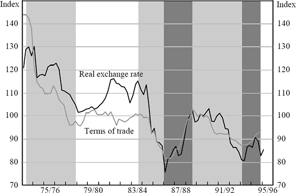
An exception can be identified in the early 1980s. This period coincides with a resources investment boom, promoted by the second OPEC oil-price shock and provides a good example of the role that expectations can play in determining movements in the exchange rate. The resources boom generated optimistic expectations about future improvements in the terms of trade and thereby, future income; the TWI appreciated despite little change in the prevailing terms of trade. Given that the anticipated improvements never eventuated, a correction in expectations contributed to the magnitude of the real TWI depreciation over 1985 and the first half of 1986.
Secondly, Australia experienced a rapid and sustained rise in net foreign liabilities over the 1980s (Figure 4).[9] Increasing net foreign liabilities, as a share of wealth, require larger balance of trade surpluses to restore equilibrium.
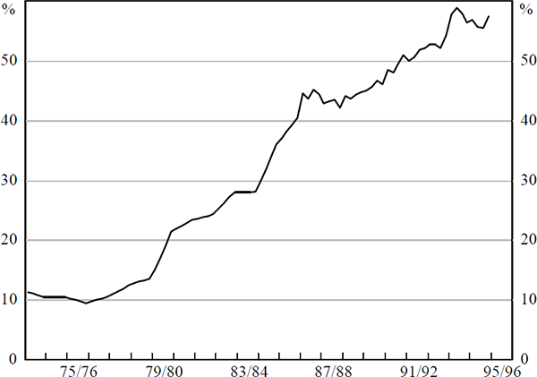
Similar to the macro-model mechanism of maintaining external balance, this may require a depreciation of the real exchange rate to attract resources into the tradeables sector. (Of course, if the real return on investment is high, the higher trade surpluses may be achieved without a real depreciation.)
Thirdly, the vast majority of the literature finds that the long-term real interest differential has the most success in obtaining significant and correctly signed estimates in exchange rate equations (Gruen and Wilkinson (1991) and BW for Australia; Isard (1988) and Shafer and Loopesko (1983) for international evidence). Long-term interest differentials are often justified on the grounds that shocks to the real exchange rate can persist for long periods and this slow reversion towards equilibrium is simply more appropriately matched by a correspondingly long-term interest rate.[10] This seems curious given that the exchange rate is considered to be an important channel through which changes in the policy-determined short-term interest rate feed through to the economy. De Kock and Deleire (1994) estimate that, post 1982 in the United States, the exchange rate accounts for roughly one-third of monetary policy transmission to output, compared to a near-negligible contribution earlier. Perhaps it is the case that earlier Australian studies did not have the benefit of a sufficiently long sample period, after the floating of the Australian dollar, over which to estimate their exchange rate models. At any rate, this seems to beg further investigation.
The real long-term interest differential in existing models could simply be replaced by a real short-term interest differential. As customarily measured – using 12-months-ended inflation rates – real short-term interest rate differentials would reflect the prevailing stance of domestic, relative to foreign, monetary policy; but they would fail to capture any market anticipation of the future paths of short-term interest rates, inflation and growth.
It is difficult to capture these forward-looking aspects in behavioural models. This seems unsatisfactory in models of the exchange rate since financial market behaviour is generally characterised by forward-looking expectations. Therefore, the novel approach taken here is to use a measure of the relative slopes of the domestic and foreign yield curves. Mishkin (1994) and Estrella and Mishkin (1995) provide evidence that the slope of the yield curve contains information about the current and expected future stance of monetary policy.[11] Inflationary expectations, and therefore expectations of the future path of short-term interest rates, are reflected in long bond yields. Although well-understood by policymakers, it is worthwhile digressing to illustrate this operational point stylistically.
Figure 5 depicts two episodes of monetary policy action in Australia. Between April and December 1987 (top panel) and from December 1990 to March 1992 (bottom panel), the operational instrument of monetary policy in Australia – the nominal cash rate – was reduced by around 5½ percentage points.
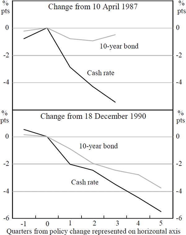
In the first episode, in 1987, the long bond yield remained relatively unchanged (falling by a small 0.48 of a percentage point). By comparison, over the early 1990s episode, the long bond yield fell by almost 4 percentage points. At this time, some progress on inflation was already widely apparent in Australia and so market expectations for future inflation may well have moderated with the reduction in the cash rate. Of course, this discussion is simplistic and ignores a number of issues, but to the extent that inflation expectations explain some of the fall in the long end of the yield curve, agents were not expecting short-rates to have to rise very much in the future. Relative to the example in 1987, the slope of the yield curve remained fairly flat. By this measure, the stance of monetary policy was relatively tighter than over the 8 months to December 1987, despite equivalent movements in the nominal cash rate.
Also of interest to policymakers is the role of fiscal policy in determining exchange rate behaviour. Rarely mentioned in earlier work on the Australian exchange rate, the impact of fiscal policy can occur through two separate channels and is theoretically ambiguous.
- Firstly, the simplest Mundell-Fleming model predicts that expansionary fiscal policy causes an appreciation of the exchange rate. The intuition for this result is that increased government spending raises demand for domestic output which, in turn, induces a currency appreciation (alternatively, increased demand exerts upward pressure on interest rates which induces capital inflow and a stronger currency). The appreciated currency reduces the value of foreign demand, which restores the original level of output.
- Secondly, fiscal policy can impact upon the exchange rate through a risk premium. Fiscal expansion may be penalised by investors who perceive an increased probability of default or expect higher inflation in the future because they believe that the incentive exists for the Government to ‘inflate’ its debt away; in order to hold Australian dollar assets, they demand a risk premium on domestic interest rates. Furthermore, it is often argued that higher government budget deficits are associated with negative sentiment on the exchange rate because they imply lower national savings and so greater net foreign liabilities in the longer run. In this way, it is argued that the exchange rate depreciates. To the extent that the negative sentiment arises because of the overall size of net foreign liabilities, rather than their public/private composition, this effect may be partly captured, over the long run, by a cumulated current account variable.
Both the monetary and fiscal policy variables discussed above seem likely to be important, in addition to the variables identified in earlier work, for explaining movements in the Australian real exchange rate. To ascertain the empirical validity of this proposition, the BW equation, being the most recent in this literature, is tested for and appears to suffer from omitted variable bias.
Table 1 summarises the results from application of the ‘rainbow test’, a member of the Ramsey (1969) RESET family of tests for the omission of unknown variables (Utts 1982).[12] The test is conducted over several post-float sample periods, when the exchange rate became a channel of transmission for monetary policy; the null hypothesis of no omitted variables is consistently rejected. The omitted variable(s) will be captured in the error process and as a consequence, the estimated coefficients in the BW equation will be both biased and inconsistent.
| Estimation period | RESET Rainbow test | Significance level | |
|---|---|---|---|
| 1984:Q1–1992:Q3 (BW 1993) |
3.11** |
F(18,10): |
0.035 |
| 1984:Q1–1995:Q2 (Updated BW sample) |
2.61** |
F(24,16): |
0.026 |
| 1985:Q1–1995:Q2 (Tarditi 1996) |
2.02* |
F(22,14): |
0.089 |
|
Notes: ** and * denote rejection of the null hypothesis of no omitted variables at the 5% and 10% significance level. |
|||
In an effort to address this bias, several modifications to the BW specification are made. Specifically, the terms of trade and cumulated current account deficit are retained. A yield gap differential replaces the long-term interest differential and takes the form:
where:
| (is−L) | measures the slope of the domestic yield curve as the difference between the domestic nominal cash rate (is) and the domestic nominal long (10 year) bond yield (iL); |
| (is-iL)* | measures the slope of the foreign yield curve using equivalent foreign interest rates (see Appendix A for details on the construction of world interest rates and Table B.2 in Appendix B for statistical confirmation of the implied restrictions in (1)). |
In addition, a role for fiscal policy is accommodated by including a measure of the change in the Commonwealth Government budget balance, expressed as a proportion of GDP (hereafter, the fiscal variable). While it would be preferable to use a cyclically-adjusted measure of the fiscal position, this was not available for Australia.[13]
3.2 The Empirical Results
Following the convention for time series methodology, the order of integration of the real exchange rate and its proposed explanatory variables is established (see Table B.3 in Appendix B for detailed statistics). To this end, the Augmented Dickey-Fuller (Dickey and Fuller 1981; Said and Dickey 1984) and Elliot, Rothenberg and Stock (1992) (DF-GLS) tests of a unit root null, together with the Kwiatkowski, Phillips, Schmidt and Shin (1992) (KPSS) test of a stationary (trend stationary) null, are employed.[14] Confirming the results of Bleaney (1993) and Gruen and Kortian (1996), these tests imply mean reversion of the Australian real exchange rate to a slowly declining trend.[15] Similar evidence of stationarity exists for other countries (see, for example, Phylaktis and Kassimatis (1994); Liu and He (1991) and Huizinga (1987)).[16] The integration tests also provide evidence that the terms of trade and other explanatory variables are I(0) processes.
Nevertheless, the analytical convenience of the unrestricted error correction framework is exploited to specify a behavioural model of the real Australian TWI exchange rate.[17] The model is specified with 4 lags of each explanatory variable in the dynamics; lower case denotes logarithms. Sequential F-tests are used to derive the following parsimonious representation:
where:
| rer | Australian real TWI exchange rate; |
| tot | terms of trade; |
| cad | cumulated current account deficit, expressed as a proportion of GDP (defined such that a current account deficit is a positive number); |
| YGAP | relative slopes of domestic and foreign yield curves as described in (1) above (see Table B.2 in Appendix B for statistical confirmation of the implied interest rate restrictions); |
| Δgdef/gdp | fiscal variable, defined as the log change in the Commonwealth Government deficit and expressed as a proportion of GDP (defined such that a budget deficit is a positive number); |
| ε | white noise error term; |
| Δ | first difference operator. |
Given the time-series properties of the data, this specification is used to distinguish different types of influences on the real exchange rate and, in this way, retains one characteristic of the macroeconomic models described in Section 2 – namely, the general framework wherein the real exchange rate – affected by speculative and cyclical factors – eventually tends toward a path determined by underlying structural factors. The macroeconomic fundamentals, identified in Section 3.1 above, set the parameters within which the exchange rate should move in the medium term and provide a pertinent framework from which to assess the appropriateness of policy settings.
The model is estimated over two sample periods; three decades of data encompass two broad exchange rate regimes in which the dynamics of the real exchange rate are unlikely to be identical. With this in mind, results for equation (2) over the post-float period (1985:Q1–1995:Q2)[18] and a longer, historical sample (1973:Q4–1995:Q2) are reported in Table 2.
| Explanatory variable | 1985:Q1–1995:Q2 | 1973:Q4–1995:Q2 |
|---|---|---|
| β: Real exchange ratet−1[19] | −0.51*** (0.12) |
−0.25*** (0.07) |
| δ: Terms of trade t−1 | 0.46*** (0.14) |
0.22*** (0.07) |
| φ: Cumulated current account deficit t−1 | −0.01 (0.05) |
−0.04** (0.02) |
| γ: Yield curve differential t−1 | 1.10*** (0.35) |
0.08 (0.21) |
 |
4.87*** {7.15} |
1.36*** {5.43} |
| θ: ΔTerms of trade t | 1.41*** (0.19) |
0.89*** (0.16) |
| α: Constant | 0.16 (0.31) |
0.09 (0.25) |
 |
0.74 | 0.35 |
| DW | 1.53 | 1.88 |
ARCH (4) test  |
1.33 [0.86] |
3.26 [0.52] |
AR (4) test  |
5.48 [0.24] |
5.19 [0.27] |
Jarque-Bera Normality test  |
2.28 [0.32] |
2.40 [0.30] |
| Rainbow test | 1.08 [0.45] |
0.84 [0.72] |
|
Notes: ** and *** denote significance at the 5% and 1% levels. Standard errors are in round brackets; probability values are in square brackets; and the F-test statistic for the joint significance of the fiscal variables is in parentheses, {}. |
||
Three points are worth noting straight away.
- As expected, it is only after the floating of the Australian dollar that the exchange rate has played a role in channelling changes in real interest rates through to the broader economy.[20]
- On the other hand, the cumulated current account deficit is only significant in explaining the real exchange rate over the fuller, historical sample period; this accords with its longer-run structural nature.[21] Over this period, the level of Australia's net foreign liabilities is estimated to have exerted some downward pressure on the real exchange rate, but this has been of a relatively small order of magnitude; a one percentage point increase in net foreign liabilities to GDP, ceteris paribus, has an estimated long run effect of ⅙ of a percentage point on the real exchange rate over this period.
- The positive coefficient on the fiscal policy variable implies a conventionally-signed Mundell-Flemming effect during the sample period.
The remainder of this section concentrates on interpretation of the results obtained from estimation of this model over the post-float period. Simple impulse response diagrams show the estimated impact of shocks to the yield curve and to the terms of trade, ceteris paribus, on the real exchange rate.
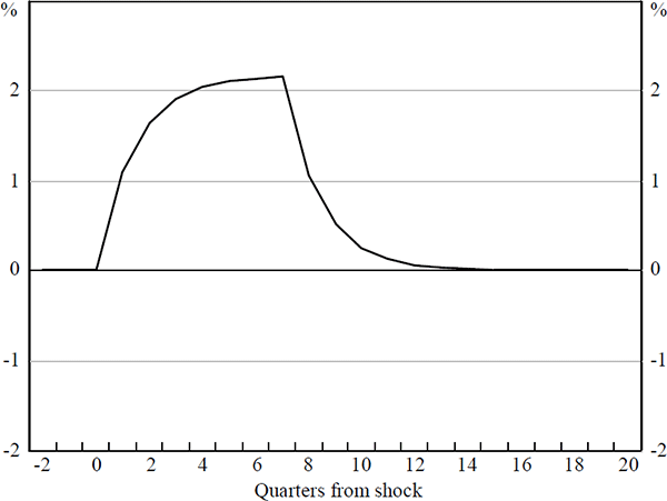
The first shock is defined as a one percentage point inversion of the Australian yield curve relative to the foreign yield curve, maintained for eight quarters. In response, the real exchange rate is estimated to appreciate by 2.2 percentage points; 76 per cent of the adjustment is complete after two quarters (Figure 6a). This gradual adjustment of the real exchange rate to an interest rate shock is quite different from the ‘jump’ responses elicited in macro models.
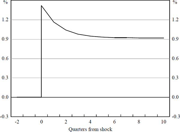
Secondly, consider a terms of trade shock. Similar to the results obtained by earlier work, a one percentage point increase in the terms of trade that is sustained for ten quarters, eventually delivers a 0.9 per cent appreciation of the real Australian exchange rate (Figure 6b). This estimated response is almost double that returned by simulation of the TRYM model discussed in Section 2. While there is some uncertainty about the operation of the short-run dynamics, a literal interpretation of the estimated model suggests an initial response of as much as 1.4 per cent.
The magnitude of the estimated real exchange rate response to terms of trade shocks is something of a puzzle. Gruen and Kortian (1996) contend that this observed historical response results from inefficiency in the foreign exchange market. They demonstrate the existence of large, variable and predictable excess returns to holding Australian assets over horizons of a year or more. This is interpreted as evidence of a relative scarcity of forward-looking foreign exchange market participants with an investment horizon of this length.
If this myopic behaviour does indeed prevail, participants in the foreign exchange market may not be adequately distinguishing between temporary, soon-to-be-reversed shocks and longer, more sustained shifts in the terms of trade. This would result in Australia's real exchange rate moving more tightly with the terms of trade than would be consistent with perfectly forward-looking investor behaviour. While the smaller responses to temporary terms of trade shocks generated by the macro models is theoretically appealing, the presence of excess returns in the foreign exchange market undermines the predictions of UIP; this condition is the central relationship determining exchange rate outcomes in the macro models.
To give some idea of the model's fit, Figure 7 compares the actual behaviour of the real Australian TWI exchange rate over the post-float period, with predicted values from this model up to the June quarter of 1995. In sample, the model fits very well.
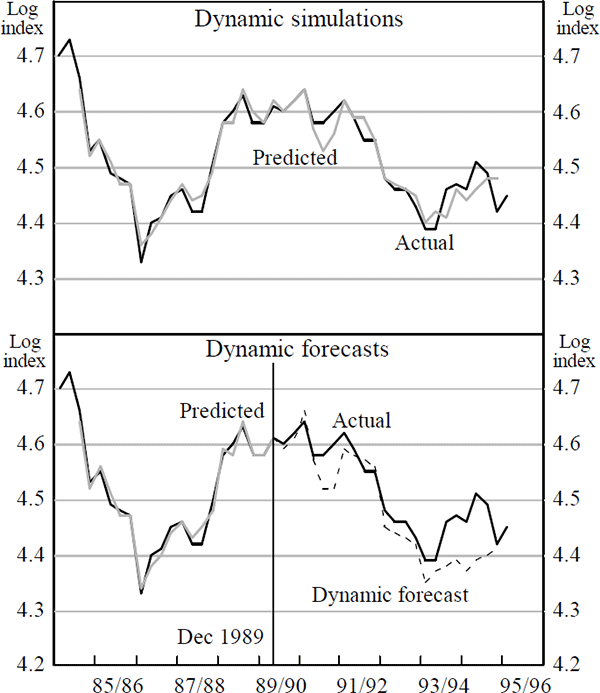
The bottom panel of Figure 7 presents the model's out-of-sample forecasts over the same period. These are obtained by re-estimating equation (2) using data to the December quarter of 1989 (or half the sample period). Subsequently, actual values of the exogenous variables are used to obtain one-step-ahead forecasts of the real exchange rate out to the end of the sample, 1995:Q2. Out-of-sample, the equation captures most of the actual movements in the real exchange rate and picks the major turning points in the early 1990s and again around the end of 1993. The tracking ability of the equation is mainly attributable to the role of the terms of trade in explaining exchange rate movements. This result is consistent with findings of a number of earlier studies. Nevertheless, the result appears at odds with standard economic theory and, as discussed above, the assumption of market efficiency.
Footnotes
This is the terms of trade for goods and services. It seems reasonable to take the terms of trade as exogenous because Australia's share of world trade is small and it exports relatively few differentiated products. Dwyer, Kent and Pease (1994) present empirical evidence for Australia. [8]
Empirical work generally uses the cumulated current account deficit as a proxy for net foreign liabilities because it abstracts from valuation effects. [9]
Isard (1983) supports the use of long (10-year) interest rate differentials on the grounds that they are convenient to interpret. As in the Australian macro models, he assumes that the expected real exchange rate in 10 years time is the equilibrium exchange rate; in this way, the long (10-year) real interest differential (corrected for any risk premium) can be interpreted as denoting the annual rate of real depreciation/appreciation of the dollar expected by the market over the next 10 years. [10]
See also Cook and Hahn (1990) for a survey of the literature and some support for the idea that parts of the yield curve are useful in forecasting interest rates; Lowe (1994) provides evidence for Australia. [11]
The ‘rainbow test’ compares estimates of the variance of the regression disturbance obtained from estimation over the relevant full sample and a truncated sub-sample; if the null hypothesis is true, both variance estimates are unbiased. The test statistic is an F-statistic, adjusted for the appropriate degrees of freedom. See Kmenta (1990, pp.454–455) for a full description of the test. It should be noted that the consequences of omitting relevant explanatory variables are the same as those of using an incorrect functional form. [12]
Typically, the government budget tends to be in surplus when the economy is growing strongly and vice versa. The fiscal variable was tested against domestic and foreign growth variables and measures of the output gap to eliminate the possibility that it was just proxying the economic cycle. The fiscal variable retained its explanatory power over both the shorter post-float period (1985:Q1–1995:Q2) and the longer, historical sample period (1973:Q4–1995:Q2). These results were not qualitatively altered when the Commonwealth Government measure of the fiscal position was replaced by a measure of the change in the public sector borrowing requirement. [13]
The null hypothesis of a unit root in the ADF and DF-GLS tests may result in a type II error; series may appear to contain a unit root because the data are insufficient to provide strong evidence for rejection of that null. This is why the KPSS test, with a null of stationarity, is also applied to the data (see Appendix B for a brief description of this test). [14]
From the perspective of modelling, the essential difference between the trend-stationary and integrated model specifications is the nature of the process driving the stochastic component, not whether the series is trended. [15]
Phylaktis and Kassimatis (1994), in examining real exchange rates in eight Pacific Basin countries (calculated using the unofficial black market exchange rates), find evidence for mean reversion which suggests a half-life of four quarters. Using amended variance ratio tests, Liu and He (1991) offer evidence that mean reversion is quicker in the developing Asian countries relative to industrialised countries. Huizinga (1987) employs spectral methods to analyse real exchange rates for ten major currencies vis-a-vis the US dollar. Various real bilateral rates against the US dollar and the pound sterling were found to be mean-reverting, but against the Japanese yen, the exchange rates were indistinguishable from random walks. [16]
In this way, this analysis recognises that in finite samples, any trend stationary process is nearly observationally equivalent to a unit root process where shocks are substantially reversed – that is, where the errors have a moving-average component with a root near minus one (or a fat-tailed distribution for the error process). And, irrespective of the order of integration of the variables, this modelling technique remains valid. [17]
The foreign exchange market is given one year after the floating of the Australian dollar in 1983:Q4 to establish its new regime; thus, estimation over the shorter sample period begins in 1985:Q1. If the entire period since the float is included in the estimation period (ie 1984:Q1–1995:Q2) then a direct role for monetary policy is no longer significant at the 10 per cent level. [18]
β measures the speed of adjustment which, for the post-float regression, implies a half life of 1 quarter; this is not unreasonable given that the real exchange rate is trend stationary. [19]
It is worth noting that the relative yield gap variable outperforms (statistically) the alternative short-term real interest differential over this sample period (see Table B.4 in Appendix B for details). [20]
This is the opposite of the BW result that the cumulated current account deficit is only significant over the shorter, post-float sample period and even then, that it is outperformed by a simple trend (see Table B.1 in Appendix B). [21]

