RDP 9608: Modelling the Australian Exchange Rate, Long Bond Yield and Inflationary Expectations 4. A Behavioural Model of the Australian Long-Term Interest Rate
November 1996
- Download the Paper 171KB
In contrast to the volume of literature on determinants of the exchange rate, work on modelling the behaviour of the Australian long bond rate is scarce. This section of the paper draws on recent work undertaken at the OECD by Orr et al., who identify a comprehensive list of the fundamental determinants of real long-term interest rates across a 17-country panel data set, including Australia. The authors also provide a succinct yet comprehensive discussion of each of these determinants. This discussion will not be repeated here. Instead, by using the ‘fundamental’ variables identifed by Orr et al, a time-series equation for the Australian ex ante real long bond rate is trialed.
This time-series specification suffers several inadequacies and raises the question of how best to transform nominal bond yields into real magnitudes. Since inflation expectations are largely unobservable, Section 4.2 of the paper spends some time exploring one possible methodology for their measurement. Estimation of a simple model of inflation, specified to endogenise shifts between a high and a low inflation regime, is used to generate forward-looking expectations. This methodology seems particularly apt for Australia, where successful inflation reduction policies in the early 1990s have been accompanied by a discrete shift in existing survey measures of inflationary expectations. The explanatory performance of this unconventional forward-looking measure is compared to an existing survey measure of inflationary expectations in a time-series model of nominal long bond rates.
4.1 The Real Bond Yield Fundamentals in Brief
I begin with the principle determinants of real long bond yields. Orr et al. list these determinants as the domestic rate of return on capital, the world real long bond yield, and various risk premia. They note that these risk premia are likely to depend on:
-
the perceived degree of each country's monetary policy commitment to price stability.
Recognising that the expectations of market participants may follow some adaptive process,
they use the existing level of inflationary expectations, conditioned on some longer-run
historical performance (the average rate of inflation over the preceding 10 years,
 ). In
this way, movements in bond yields relative to changes in current inflationary expectations
will depend on the weight that investors attribute to Australia's relatively poorer
historical inflation performance;
). In
this way, movements in bond yields relative to changes in current inflationary expectations
will depend on the weight that investors attribute to Australia's relatively poorer
historical inflation performance;
- the expected sustainability of government fiscal and net external debt positions. Orr et al. measure these with the ratios of government budget positions and cumulated current account deficits, respectively, to GDP; and
- some undiversifiable domestic portfolio risk associated with holding bonds.[22]
Following the time-series methodology outlined in Section 3, the real long bond yield, r, deflated simply, first of all, with (annualised) quarterly underlying inflation rates, is determined by an unrestricted error correction model.[23] Tests of the order of integration of each variable are presented in Table C.1 in Appendix C. Four lags of each of the differenced ‘fundamental’ variables, together with domestic growth, were included in the initial dynamic specification of the model; F-tests were then used to derive the parsimonious final model:
where:
| rt | real Australian 10-year bond yield, deflated with annualised quarterly underlying inflation rates; |
 |
the average rate of inflation over the preceding 10 years; |
| Et(π) | current inflationary expectations, generated by a Hodrick-Prescott filter of the GDP deflator; |
| RetCap | return on capital, measured as in Orr et al., as the ratio of gross operating surplus of private corporate trading enterprises to that sector's capital stock; |
| GDef | Commonwealth Government Budget deficit, expressed as a proportion of GDP (a deficit is denoted as a positive number); |
| g | domestic GDP growth, measured with the four-quarter-ended growth rate of GDP; |
| εt | white noise error term; |
| Δ | difference operator. |
The estimation results are presented in Table 3 (see Table C.2 in Appendix C for the full dynamics). Despite the richness of the Orr et al. cross-sectional specification, only the return on capital and the inflation credibility risk premium were found to be significant fundamental determinants of the Australian real bond yield in this time-series model.
| Explanatory variable | Coefficient (Standard error) | ||
|---|---|---|---|
| Speed of adjustment parameter | −0.513*** | (0.10) | |
| Return on capital | 0.164*** | (0.04) | |
Inflation term :  |
0.256*** | (0.08) | |
 |
0.60 | ||
| DW | 1.76 | ||
| ARCH test |  |
0.882 | [0.347] |
| AR (4) test |  |
3.28 | [0.512] |
| Jarque-Bera Normality test | |
0.96 | [0.618] |
|
Notes: *** denotes significance at the 1% level. Standard errors are reported in round brackets; probability values are in square brackets. |
|||
A one percentage point rise in the domestic return on capital in this model implies an eventual increase in the real long bond yield of about ⅓ of a percentage point; this compares to around ¼ per cent in the Orr et al. estimation.
While the inflation differential variable,  , has some appeal for
estimation with panel data, its appropriateness within this time-series framework is difficult
to justify. This is because, by construction, the real bond yield will often be relatively high
in periods when the current (expected) rate of inflation is low; this will also be true of the
inflation variable. That is, the existence of some mean reversion in inflation would generate
this positive, significant coefficient on the inflation differential variable.
, has some appeal for
estimation with panel data, its appropriateness within this time-series framework is difficult
to justify. This is because, by construction, the real bond yield will often be relatively high
in periods when the current (expected) rate of inflation is low; this will also be true of the
inflation variable. That is, the existence of some mean reversion in inflation would generate
this positive, significant coefficient on the inflation differential variable.
The fit of the model is represented in the top panel of Figure 8. Out-of-sample forecasts are obtained by estimating the model to December 1991; actual values of the exogenous variables are then used to forecast the real long bond yield forward through time. The results are presented in the lower panel of Figure 8.
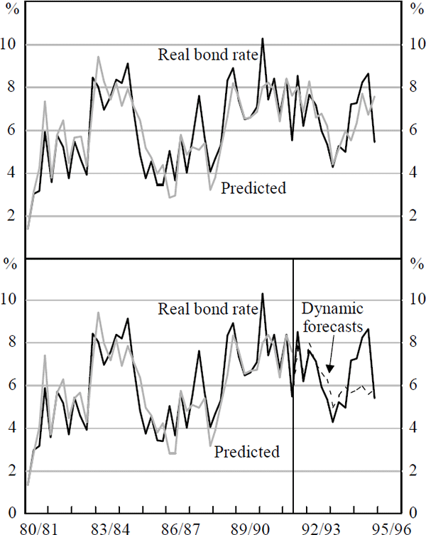
The model predicts the fall in the real long bond yield over the early 1990s and its trough in 1993. However, it fails to anticipate the extent of the rise in the real bond yield over the course of 1994, suggesting, perhaps, that the world-wide bond market sell-off was not completely consistent with fundamentals. Despite the fact that a similar pattern was documented in most OECD countries over 1994, the panel estimation in Orr et al. also fails to predict bond yield behaviour over this period.
Given the reservations with the model's (likely spurious) dependence on the inflation
differential term, , it may be the case
that the dependent variable, measured as it is, with backward-looking inflationary expectations,
is not an adequate measure of the ex ante real long bond yield. The remainder of this
section concentrates on one alternative method of constructing a forward-looking measure of
inflation expectations for inclusion in a model of Australian long bond yields.
4.2 Measuring Inflationary Expectations
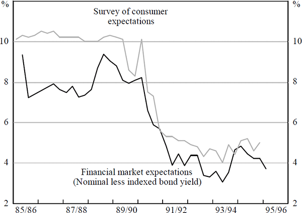
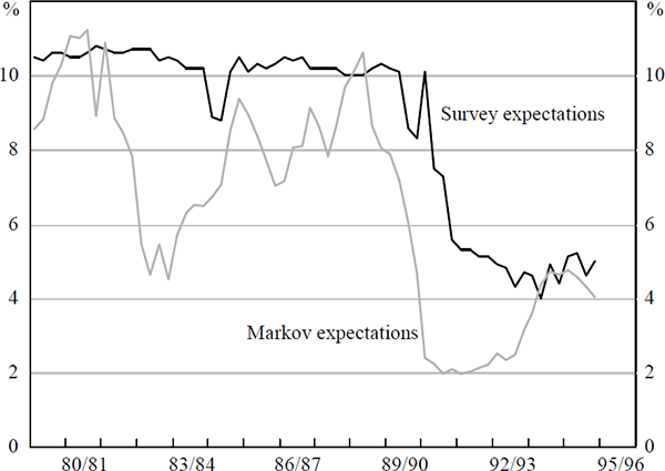
The gap between nominal and indexed 10-year bond yields is often used to estimate financial market expectations of the average rate of inflation over the next 10 years. However, in Australia's case, the indexed bond market has only very recently become liquid; historically, indexed bonds were held in concentrated parcels and were not actively traded in a secondary market at all until 1993. An alternative measure of inflationary expectations is available from the Westpac Bank and the Melbourne Institute. A random selection of 1,200 adults aged 18 and above, sampled Australia-wide, are asked to respond to a question about how much they expect prices to rise over the next twelve months; their responses are weighted to reflect population distribution. The disadvantage of this consumer survey series for models of the long bond rate is that it asks about inflationary expectations over the next 12 months – not over the next 10 years. Perhaps more importantly, the expectations of consumers might differ from those of financial market participants (Figure 9).
This paper proposes a different approach to measuring expectations which exploits the Markov-switching technique and endogenises shifts in the inflation process through time.[24] In brief, this methodology allows the process of inflation to be characterised by two different regimes, the first identified by relatively high inflation; the second, by relatively low inflation. Switches between these states are based on a probabilistic process.[25] Maximum likelihood estimation of the two-state model returns a probability that inflation is in one or other of these regimes. This is used to construct a probability-weighted n-period-ahead inflationary expectations series which is, by its nature, forward looking. Thus constructed, this series is found to be superior to its survey alternative in a model of the nominal bond yield (Section 4.3).
More specifically, inflation is specified to depend on its own past values and forward-looking measures of the output gap (itself measured by a Hodrick-Prescott filter on GDP(A)). Three forecasting methods are tried.
-
Firstly, agents are assumed to have perfect foresight so that they know the output gap existing in the period over which their inflationary forecast is relevant. In this case, the probability-weighted inflationary expectations series is a function of lagged inflation and the actual future output gap; this ‘perfect-foresight Markov measure’ is denoted EPFt(πt+n):
In this way, inflationary expectations over the next year (n=four quarters) would be EPFt(πt+4); over the next 10 years, EPFt (πt+40).
-
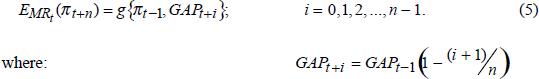
Alternatively, the assumption of perfect foresight can be relaxed so that inflationary expectations are a function of lagged inflation and a mean-reverting output gap; this ‘mean-reverting Markov measure’ is denoted EMRt (πt+n):
In this way, n=four quarters is roughly consistent with a four to five year business cycle; at any point in time, t, the output gap is not known (although GAPt−1 is known), but is expected to close within five quarters.
- Finally, since similar analysis in the literature has commonly been univariate, the output gap is excluded altogether (this worsens the fit of the model but leaves the general dynamics relatively unchanged).

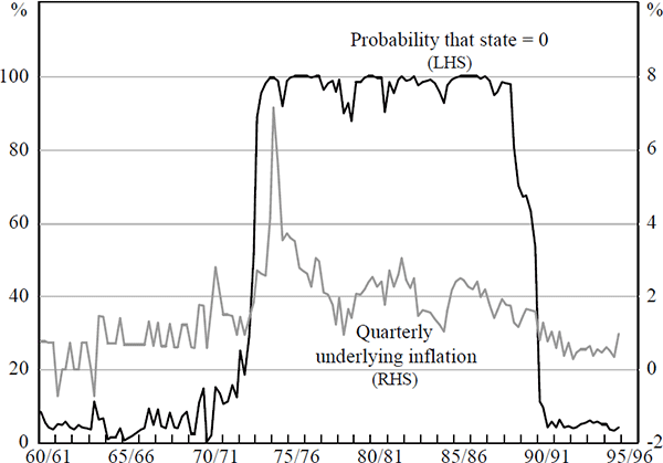
Quarterly data from the past 35 years (1959:Q4–1995:Q2) are used to estimate the model parameters with maximum likelihood techniques. For convenience, only the results from estimation of the first specification, EPFt (πt+n), which assumes perfect foresight of the output gap, are presented below. State 0 identifies the 1970s and 1980s as episodes of relatively high inflation in Australia and the estimated model describes underlying inflation as a persistent (but not integrated) process around a mean of 8.7 per cent. State 1 identifies the 1960s and 1990s as low inflation regimes where shocks are less persistent and inflation reverts to a mean of 3.3 per cent.
| State 0: High inflation regime* | State 1: Low inflation regime |
|---|---|
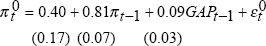 |
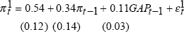 |
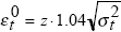 |
 |
| (0.14) | |
| p(st = 0| st–1 = 0) = 0.989 | p(st = 1| st–1 = 1) = 0.980 |
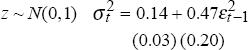 |
|
|
* Figures in parenthesis below the parameter estimates are standard errors. The notation follows the standard for ARCH and st denotes the state (either 0 or 1) in period t. |
|
Figure 10 illustrates the probability of being in the high inflation state, 0, at each point in time. It is this series which is used to appropriately weight one-step-ahead forecasts from the inflation models of state 0 and state 1 to construct what will be referred to as the ‘Markov inflationary expectations series’.
This approach has two advantages. It explicitly incorporates the forward-looking behaviour customarily associated with financial market participants and assumed in the macro-model approach. Furthermore, this method can deliver a longer-horizon measure of inflationary expectations, η periods ahead, as per (4) or (5). These n-step-ahead estimates embody more realistic, behavioural processes than the simple log linear interpolated values used in the macro models. Expectations two-years-ahead, as well as one-year-ahead, are calculated.
It is clear from Figure 11 that the behaviour of the Markov expectations series is quite distinct from that of the consumer survey measure. For exposition, only the Markov one-year-ahead inflationary expectations, generated by agents with perfect foresight of the output gap, EPFt (πt+4), are illustrated in Figure 11. The alternative, mean-reverting output gap specification and the two-year-ahead forecasts of Markov expectations exhibit similar patterns and timing.
4.3 Empirical Results for the Long Bond Yield Equation With Forward-Looking Inflationary Expectations
The relevance of the various forward-looking Markov expectations series, in contrast to the survey measure of consumer expectations, is examined for explaining movements in the nominal bond yield. This is achieved by estimating an unrestricted ECM of the form:

where:
| it | nominal 10-year bond yield; |
 |
estimated average rate of inflation expected over the next 10 years proxied either by one of the Markov measures of inflation expectations or the consumer survey measure; |
| Z | vector of explanatory variables for the real 10-year bond yield as described by Orr et al. and discussed in Section 4.1 above; of all the variables listed in Orr et al., only the return on capital and, in one case, the foreign real long bond yield were found to be statistically significant Z variables. |
| X | vector of dynamics; |
| εt | white noise error term. |
Four lags of each of the differenced explanatory variables were initially included in the
dynamic specification of the model; F-tests were then used to derive the parsimonious final
model. Table 4 summarises the results from estimation of (6) using the competing measures of
.
 |
Z | ||||||
|---|---|---|---|---|---|---|---|
| Model No. |
Measure of |
β (t-statistic) |
α Speed of adjustment (t-stat) |
γo Return on capital (t-stat) |
γ1 r* (t-stat) |
 |
H0: α = −β (p-value) |
| 1 |  |
0.204 (4.80) |
−0.241 (4.36) |
0.079 (2.68) |
0.13 (1.90) |
0.332 | 0.61 |
| 2 |  |
0.223 (4.10) |
−0.226 (4.38) |
0.083 (2.97) |
— |
0.284 | 0.93 |
| 3 | Survey |
0.262 (3.09) |
−0.299 (3.47) |
0.083 (2.31) |
— |
0.271 | 0.33 |
| 4 |  |
0.091 (2.05) |
−0.065 (2.95) |
— |
— |
0.216 | 0.32 |
| 5 |  |
0.245 (3.21) |
−0.210 (3.61) |
0.066 (2.33) |
— |
0.214 | 0.44 |
The Markov one-year-ahead inflationary expectations measure, calculated using the assumption of
perfect foresight for the output gap,  , was found to have the
greatest explanatory power for movements in the nominal long bond yield (Model No. 1); it
clearly outperforms the survey measure (Model No. 3).
, was found to have the
greatest explanatory power for movements in the nominal long bond yield (Model No. 1); it
clearly outperforms the survey measure (Model No. 3).
The alternative Markov measure – which is based on an assumption of mean-reversion in the
output gap rather than perfect foresight – but calculated with an equivalent one-year
forecast horizon,  , also performed better than the survey measure;
this is Model No. 2. However, in this specification, the real long foreign bond yield became
insignificant.
, also performed better than the survey measure;
this is Model No. 2. However, in this specification, the real long foreign bond yield became
insignificant.
Two-year-ahead Markov expectations,  and ,
in Models No. 3 and 4, respectively, were slightly less significant; the foreign long bond yield
was insignificant in these equations as well.
and ,
in Models No. 3 and 4, respectively, were slightly less significant; the foreign long bond yield
was insignificant in these equations as well.
The remainder of this section concentrates on the results obtained from Model No. l's specification (see Table C.3 in Appendix C for the full estimated dynamics):
where:
| it | nominal Australian 10-year bond yield; |
| EPFt(πt+4) | Markov model estimates of inflationary expectations as defined in (4) above or consumer survey measure; |
| RetCap | return on capital; |
| r* | US real 10-year bond rate; |
| g | domestic GDP growth; |
| εt | white noise error term; |
| Δ | difference operator. |
Full-sample predictions from this very simple nominal long bond yield equation fit the actual data very well (Figure 12).
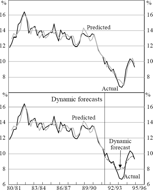
As in Section 4.1, out-of-sample forecasts were obtained by estimating the model to December 1991; actual values of the exogeneous variables were then used to forecast the nominal long bond yield forward in time. The model anticipates the turning point in bond yields in late 1993 as well as their subsequent pick-up over 1994, presumably because it contains the foreign bond yield (r*); the other models did not.
The null hypothesis in the final column of Table 4 tests that the Fisher Hypothesis holds, such that movements in inflationary expectations are matched one-for-one by movements in the nominal interest rate. This restriction is necessary for valid reparameterisation of Model No. 1 (equation (7)) as a real bond yield equation; the null hypothesis could not be rejected. Trivially, additional restrictions are also accepted such that this model, re-estimated as a real bond yield equation, delivers the same parameter estimates on the Z variables.
In this way, while equation (3) in Section 4.1, presented a model of the real 10-year bond yield, deflated with backward-looking expectations, equation (7) provides an alternative model wherein real yields are constructed using a forward-looking Markov measure of expectations. The main features of this latter model are listed below.
The Australian nominal long bond yield reacts to a change in inflationary expectations with a lag (bottom panel of Figure 13). In contrast, a permanent 1 percentage point rise in the US real long bond rate, ceteris paribus, causes the Australian real long bond yield to react instantaneously; by the second quarter after the shock, the domestic long bond yield would be around 0.54 of a percentage point higher (panel 2, Figure 13; this is larger than the 0.30 of a percentage point implied by the Orr et al. cross-section estimates for Australia).
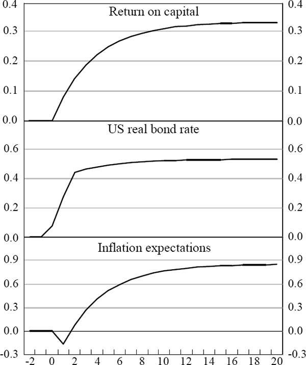
Consistent with the result obtained from estimation of equation (3), a permanent 1 percentage point improvement in the return on Australian capital raises the domestic real yield by around ⅓ of a percentage point; this response occurs more slowly than that estimated for a change in the US real rate (panel 1, Figure 13).
Footnotes
It may also be the case that some degree of liquidity risk exists for Australia, due to a relatively shallow bond market. It is reasonable to expect that this risk is declining over time as the market matures and deepens. [22]
Annualised quarterly inflation rates are used to avoid the introduction of autocorrelation. [23]
Initial work with Markov-switching models was done by Hamilton (1989,1990) with applications to business cycles. Recent work by Evans and Wachtel (1993) and Laxton, Ricketts and Rose (1994) (and Simon (1996) for Australia) has applied the technique to inflation with a view to examining the issue of central bank credibility. The Gauss programme used for estimation of the Markov switching model is an adaption of that used by Hamilton (1989) and Goodwin (1993) and I thank Thomas Goodwin for generously providing me with the computor code. [24]
A Markov process is one where the (fixed) probability of being in a particular state is only dependent upon what the state was last period. [25]