RDP 9607: Towards an Understanding of Australia's Co-Movement with Foreign Business Cycles 3. The Foreign Business Cycle and Australian Exports
November 1996
- Download the Paper 149KB
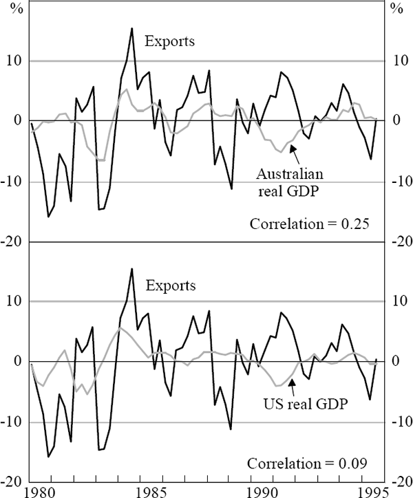
This section looks at the impact of foreign activity on Australian exports. Figure 2 shows the cycles in exports, Australian GDP and US GDP. The correlations between Australian exports and the two countries' GDPs are low, at 0.25 and 0.09 respectively. At first sight these low correlations seem to imply that foreign activity is not important for Australia's exports and that exports, in turn, are not determining Australian activity. However, this analysis ignores the fact that exports may be driven by movements in both foreign and domestic demand. By recognising this, the following ‘exports’ mechanism for the transmission of business cycles can be posited. Suppose that a high level of world activity increases the demand for Australian exports and, furthermore, that a high level of domestic activity reduces exports. The latter assumption follows because Australian producers divert exports to satisfy domestic demand. As a result, the net effect on exports of an increase in domestic and foreign activity may be small. Consequently, the correlation between exports and either domestic or foreign activity will appear low, even though Australia's exports are in part dependent on foreign activity.

Notes: The figures show the deviation from the sample average four-quarter-ended growth in each series.
While the idea that increased foreign activity increases exports is straightforward, the idea that domestic demand decreases exports is less so. Menzies and Heenan (1993) argue that producers switch in the short run between foreign and domestic markets depending on domestic activity. However, domestic activity also affects the level of exports in the long run for the following reason. As a first approximation, the trend growth in output for an economy is determined by supply factors such as capital accumulation, growth in the workforce and changes in technology. If technological progress is largely independent of export growth, then faster growth in exports must be at the expense of slower growth in that part of output which is consumed domestically.[9] In the short run this is also true but possibly less clear cut if there are idle resources.[10] However, in general, a surge in domestic demand will be satisfied partly by increased production and imports, but also partly by reduced exports. It is for this reason that we argue that there may be a long-run relationship between exports, domestic output consumed domestically, and foreign output.
Having characterised the long-run determinants of Australian exports in this way, the following unrestricted error-correction model of exports is estimated:
where the level of exports x is determined in the long run by the level of domestically consumed output ydc (equivalent to GDP less exports), the level of foreign output yf, and a time trend to capture differences in domestic and foreign output trends and structural shifts towards exports in the Australian economy. Short-run influences on exports include changes in the terms of trade tot and the real exchange rate rer.[11]
Two alternative measures of export prices were also investigated. The first was the relative price of exportable to non-traded goods. The second was the ratio of the terms of trade to the real exchange rate.[12] Both measures were incorporated in a general dynamic structure and found to be either insignificant or, as above, did not display the expected sign and so were not reported.
Before estimating the models, the time series properties of the data were investigated.[13] We find that domestically consumed output and foreign output are best characterised as I(1) variables while first differences of these variables and the remaining explanatory variables are best described as stationary, I(0) series. There is some evidence that exports are trend-stationary. However, we proceed under the assumption that exports are non-stationary.[14]
The results of estimating equation 2 are reported in Table 3.[15] Model (1) uses US GDP as
the measure of foreign output, models (2) and (3) use OECD GDP, and models (4) and (5) use
export-markets' GDP. Model (1′) will be discussed later. Exports, domestically
consumed output and foreign output are cointegrated only in the model using US GDP. In the OECD
and export-markets models (2 and 4), domestically consumed output does not enter the long-run
relationship. Excluding this variable fails to improve either of these models (3 and 5). While
not reported, a strong cointegrating relationship can be found between exports and either OECD
or export-markets' GDP if the trend is also excluded. However, the models have less than
half the explanatory power of the US based models as measured by  .
.
| United States | OECD | Export markets | |||||
|---|---|---|---|---|---|---|---|
| Lag | (1) | (1′) | (2) | (3) | (4) | (5) | |
| Constant | 5.935 (3.36) |
7.86 (4.20) |
−3.704 (−2.85) |
1.788 (0.69) |
3.187 (1.87) |
3.008 (2.12) |
|
| Exports | 1 |
−0.566 (−6.13) |
−0.556 (−6.31) |
−0.295 (−3.22) |
−0.398 (−4.42) |
−0.378 (−4.25) |
−0.387 (−4.39) |
| Domestically consumed GDP | 1 |
−1.007 (−3.52) |
−1.183 (−4.19) |
−0.286 (−1.22) |
−0.292 (−1.54) |
||
| Foreign GDP | 1 |
1.207 (3.64) |
1.197 (3.79) |
1.019 (2.88) |
0.189 (0.66) |
0.817 (4.01) |
0.106 (0.33) |
| Trend | 0.008 (4.65) |
0.009 (5.34) |
0.006 (2.70) |
0.006 (1.70) |
|||
| Domestically consumed GDP (log change) |
0 to 2 |
0.952 {0.000} |
1.068 {0.000} |
0.883 {0.019} |
1.244 {0.005} |
||
| Foreign GDP (log change) |
1 |
−1.740 (−2.99) |
−1.909 (−3.42) |
||||
| Japanese GDP (log change) |
0 |
1.397 (2.35) |
|||||
| Terms of trade (log change) |
1 to 4 |
−0.717 {0.060} |
−0.693 {0.034} |
−0.753 {0.142} |
−0.688 {0.107} |
−1.055 {0.073} |
−0.693 {0.114} |
| Real exchange rate (log change) |
1 to 4 |
0.396 {0.043} |
0.380 {0.020} |
0.118 {0.147} |
0.282 {0.188} |
0.237 {0.136} |
0.297 {0.195} |
| Long-run relationship | |||||||
| Australian GDP less exports | −1.779 | −2.129 | −0.972 | −0.773 | |||
| Foreign GDP | 2.133 | 2.152 | 3.458 | 0.475 | 2.164 | 0.275 | |
| Trend | 0.013 | 0.015 | 0.015 | 0.015 | |||
| Joint significance of terms of trade and real exchange rate | 1.746 {0.114} |
2.051 {0.062} |
1.352 {0.242} |
1.218 {0.308} |
1.592 {0.153} |
1.197 {0.320} |
|
| Diagnostics of residuals | |||||||
 |
0.499 | 0.545 | 0.271 | 0.262 | 0.360 | 0.257 | |
| LM (1)(b) | 0.115 {0.735} |
0.289 {0.591} |
0.306 {0.580} |
0.271 {0.603} |
0.097 {0.755} |
0.257 {0.612} |
|
| Standard error of equation | 0.027 | 0.025 | 0.032 | 0.032 | 0.030 | 0.032 | |
| DW | 1.90 | 2.05 | 1.85 | 1.99 | 1.98 | 2.00 | |
Notes: (a) Each model was initially estimated with 4 lags of the
short-run variables. Insignificant variables were then eliminated following
individual exclusion tests. Finally, all the eliminated variables were tested for
joint significance and rejected. Numbers in parentheses () are t-statistics and
numbers in brackets {} are probability values for the joint test that all the lags
can be excluded. The distribution of the t-statistics on the level variables in the
model lie between a N(0, 1) and a Dickey Fuller distribution (See Kremers et al. 1992). **, *, and # denote significance at
the 1%, 5%, and 10% levels respectively. |
|||||||
The relative performance of these models is counter-intuitive. In an exports equation it would
be expected that the export market and OECD models would outperform the US model, because the US
only accounts for around 10 per cent of Australia's export market. However, the cycle in
Australia's exports will depend not only on a country's export share, but also on its
output elasticity of demand for Australia's exports,  . When
  , Australia's
exports are insensitive to the business cycle in that country. For
  ,
Australia's exports and that country's business cycle will be positively correlated.
Countries with a high elasticity of demand will have a large impact on Australia's exports
over their business cycle. Conversely, countries with a low or negative elasticity of demand
will have little or even a ‘perverse’ negative impact on Australia's exports
over their business cycle.
Table 4 shows, for some of our major trading partners, the correlation between Australian exports to a particular country and its business cycle. A large positive correlation indicates a high output elasticity of demand for Australia's exports. Among the countries with the highest positive correlations are Japan and the US; Australia's two largest export partners. These results may reflect Australia's role as a major supplier of inputs for the Japanese economy, and that the US economy is relatively open. A reasonably high correlation is also found with the NIEs. In contrast, among the lowest correlations are those with countries within Europe, which may reflect less open markets. The impact of changes in activity in these countries on Australia's exports will, on average, be much lower. This helps to explain why the OECD-based model does worse than the US-based model, as the OECD-wide measure of foreign activity contains countries which have low or negative output elasticity of demand for Australia's exports. As a result, demand for Australia's exports will depend not only on OECD activity, but also on the composition of that activity. A similar argument applies to the export-markets model, since this gives weight to countries with a high average share of Australia's exports rather than to those whose demand for Australian exports is highly responsive to the business cycle.
| Japan | US | NZ | South Korea | UK | Singapore | Taiwan | |
|---|---|---|---|---|---|---|---|
| Correlation coefficient | 0.69 | 0.72 | 0.44 | 0.23 | 0.18 | 0.69 | 0.57 |
| Average export share (%) | 26.50 | 10.40 | 5.20 | 4.70 | 3.90 | 3.60 | 3.30 |
| Hong Kong | Germany | Italy | France | Canada | EU | NIEs | |
| Correlation coefficient | 0.70 | −0.63 | 0.74 | 0.14 | 0.23 | 0.32 | 0.60 |
| Average export share (%) | 3.00 | 2.40 | 2.00 | 1.9 | 1.60 | 13.90 | 14.50 |
Notes: Data are for the period 1982–1994 for NZ and for the period 1981–1994 for Taiwan and the NIEs. The logarithms of the series are detrended using linear trends. The exports series were detrended to remove structural reasons for the change in exports over the past 14 years and to ensure the series are stationary. The NIEs are Hong Kong, South Korea, Singapore, and Taiwan. |
|||||||
Given that Table 4 suggests that Japan's output elasticity of demand for Australian exports is high, the US-based model was re-estimated using US and Japanese GDP. While the level of Japanese GDP is insignificant in the long-run relationship, the contemporaneous change in Japanese GDP has a positive and significant impact on Australia's exports. These estimates are reported as Model (1′) in Table 3, which is now referred to as the ‘preferred’ model.
Turning to the short-run specification of the preferred model, we find that the terms of trade has little effect on exports and its sign is opposite to that expected. This may be because the industries which respond to the prices which drive the cycle in Australia's terms of trade are agricultural and resource based which are constrained by the weather or long-term contracts. The impact of the terms of trade on exports, therefore, is more diffuse and long-term. A higher terms of trade may well lead to higher investment and exports, but the lead time varies and depends, in part, on the perceived permanence of the change in export prices. In contrast, it has been shown that the terms of trade appears to have a large, positive and relatively rapid impact on domestic demand.[16] The model, therefore, may not be able to distinguish between the more rapid negative impact on exports through domestic demand, and the more long-term positive price effect. A similar explanation can be invoked to explain the persistent unexpected sign to the real exchange rate variable.
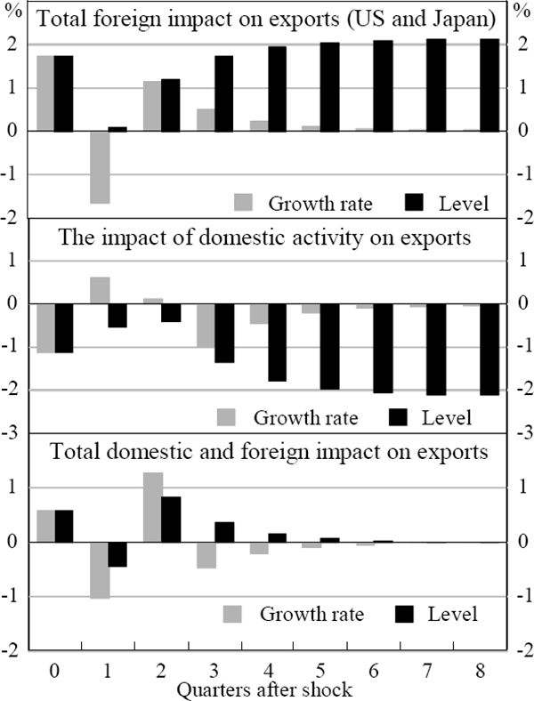
To look at the short-run impact of domestically consumed output and foreign activity on exports, we can use impulse response functions generated from the preferred model. The effects on exports of permanent shocks to domestically consumed output, US and Japanese GDP are shown in Figure 3:[17] higher foreign activity raises the level of exports while higher domestically consumed output reduces it. The net effect of a simultaneous shock to both variables is minimal change in the level of exports in the long run.[18] However, in the short run, the net impact generally increases exports. The impulse response functions imply that if the shocks to foreign and domestic activity are not highly correlated then the impact on exports and GDP will be large. However, if the shocks are highly correlated, then the net impact on exports and GDP, although positive, will be considerably reduced.

Note: The shocks to the level of domestically consumed GDP, US GDP and Japanese GDP are 1%, 0.98% and 1.23% respectively.
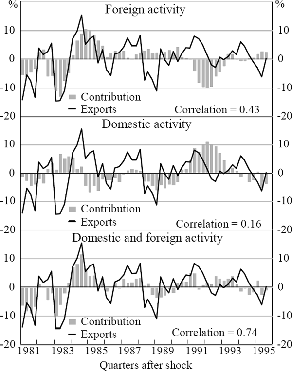
Using the preferred model we can also disentangle the historical impact of the foreign and domestic business cycles on exports. The top panel of Figure 4 shows the impact that deviations from the average growth in foreign GDP (US and Japanese) has had on exports over the sample. The impact is large and persistent. Similarly, the second panel shows the estimated impact of deviations from average growth in domestically consumed output on exports. Periods of high domestic activity serve to reduce exports. The third panel combines the effects of both the domestic and foreign business cycles on Australian exports. A large part of the cycle in exports can now be explained by the combination of these activity variables.[19]

Note: The export growth rate is the de-meaned four-quarter-ended growth in exports. The contributions are calculated as follows. Predicted values for export growth are calculated using the actual values of the exogenous variables and the predicted level of exports. Predicted values are also calculated holding a particular exogenous variable to its sample average growth rate or level over the entire sample. The contribution of that exogenous variable is then the difference between these predicted values.
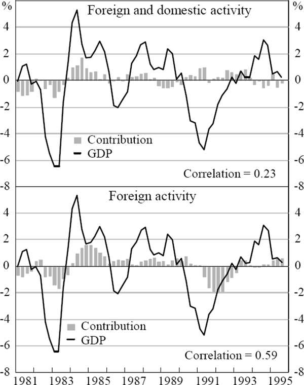
At the beginning of this section it was argued that because both domestic and foreign activity affect exports, the correlation between domestic activity alone and exports is likely to be low. The top panel of Figure 5 shows the total direct contribution to the growth in Australian GDP from domestic and foreign activity through the export channel.[20] The correlation is low, and it does not appear to explain the cycle in Australian GDP. Therefore, the export cycle, when driven by shocks to foreign and domestic activity, is a poor explanator of domestic activity. However, it was also argued above that this does not imply that foreign activity does not influence Australian activity through exports. The lower panel shows the direct contribution to domestic activity of that component of exports which is the result of the cycle in foreign activity alone. This is equivalent to removing from exports the feedback from domestic activity. Now the explanation of domestic activity is more substantial. We conclude, therefore, that foreign activity does influence domestic activity via an exports channel.

Notes: The export growth rate is the de-meaned four-quarter-ended growth in exports. Contributions to GDP growth are calculated by multiplying the contributions to export growth by the share of exports in GDP.
Footnotes
This is not as bleak as it sounds. All else equal, increased exports may have little effect on Australia's total output but still improve the standard of living. If we sell exports and buy imports we reveal that we value the imports more than the exports. [9]
The correlation between four-quarter-ended growth in exports and domestically consumed GDP (ie GDP less exports) is −0.16. [10]
See Appendix D for details of the data series. [11]
The ratio of the terms of trade (TOT) to the real exchange rate (RER) is:  where Pi is the price index and i = x, m, f, d
represents exports, imports, and foreign and domestic consumption. The ratio, therefore,
reflects changes in the relative price of exports to domestic prices compared with
changes in the relative price of imports to foreign prices.
[12]
See Appendix E for tests of the time series characteristics of the data. [13]
Interpretations of the results differ somewhat under the alternative characterisations of exports. If exports are non-stationary, equation (2) specifies the adjustment of exports to deviations from the cointegrating relationship between exports, domestically consumed output and foreign output. Alternatively, if exports exhibit trend growth, deviations from trend growth will be determined by deviations from the cointegrating relationship between the activity variables. [14]
In the model, it is assumed that ydc and yf are weakly exogenous. This assumption is supported by single equation error-correction models where deviations from the long-run relationship between x, and ydc yf impact only on exports. [15]
See Downes et al. (1994) and Gruen and Shuetrim (1994). [16]
The impulse response is for a 1 per cent permanent shock to the level of domestically consumed GDP. The shocks to the levels of foreign GDP are in the ratio of their respective average growth rates of GDP to that of Australia's growth in domestically consumed GDP. [17]
This may be considered a visual ‘test’ of the long-run condition that domestic and foreign economic cycles have no impact on the level of exports in the long run. That is, trend growth in exports is the result of ‘supply’ factors alone and captured by the linear time trend. [18]
Closer inspection of Figure 4 reveals that the explanatory power of the model may have diminished after the mid 1980s. However, if we re-estimate equation (2) over a more recent sample (say 1985:Q4 to 1995:Q3), the results are qualitatively similar. Results are not reported as the sample is too short to generate meaningful long-run parameter estimates. [19]
The contribution of exports to the growth in GDP is calculated by multiplying the export growth due to activity by the export share in GDP in the period before. [20]
