RDP 9606: The Information Content of Financial Aggregates in Australia 5. Out-Of-Sample Forecasting
November 1996
- Download the Paper 279KB
5.1 Out-Of-Sample Overview
The in-sample tests of the previous section suggest that certain financial aggregates may have limited usefulness in forecasting output and inflation in real life situations. But Cecchetti (1995, p. 199) argues: ‘Whether a model fits well in-sample tells us virtually nothing about its out-of-sample forecasting ability.’ If money is useful for explaining subsequent variations in prices and/or output within the sample, that fact does not indicate that the variable will be useful for forecasting in real time (when all future values are unknown). In this section, we use out-of-sample forecasts to compare the relative accuracy of real GDP and CPI forecasts from VAR models that contain monetary aggregates with those that do not.
There are several inadequacies of in-sample evaluation techniques for the purpose of determining the relevant information content of financial aggregates. The test statistics from the VAR (F-tests) indicate whether the lags of the financial aggregates aid in the forecast of output growth and inflation one period into the future. Although these tests are often informative about the explanatory power of the data series, policymakers have a longer time horizon than one quarter. The variance decomposition evidence indicates the information content of financial variables for longer forecast horizons, and thus overcomes this short-horizon issue. The results of the variance decomposition exercises, however, are heavily dependent on the causal ordering that is imposed on the data, and the parameter estimates are generated using data unavailable at the time of the forecast. To mimic more closely the realtime forecasting problem faced by policymakers, we employ a series of out-of-sample forecasting exercises.[19] The forecasts are evaluated using an eight-quarter forecast horizon, likely to be more representative of the horizon taken into account in policy formulation. The forecasts begin in 1984, giving 38 overlapping observations of an eight period out-of-sample forecast.
Forecasts of a VAR out-of-sample are dynamic forecasts that only use information available at the time of the forecast to predict movements in the data series in the VAR for the desired number of periods in the future (eight in our case). They are dynamic in the sense that all variables in the system must be forecast jointly in order to produce a sequence of forecasts for the variables of interest. For example, forecasting two periods into the future in an approximately real-time setting implies that in order to generate a forecast for the second period out, the VAR must use the forecasts one period out as right-hand side variables. Given that the VAR model employs four lags of the data, forecasts of five periods or more rely only on forecasts of the dependent variables as the right-hand side variables.[20]
Under the assumption that all variables in the model are available at approximately the same time, the forecasting model cannot exploit contemporaneous relationships among financial aggregates and the variables of interest. Unlike structural simultaneous equations models, there are no exogenous variables to ‘choose’. Simultaneous equation models generate forecasts conditional on the path of the exogenous variables, values that may be chosen or may be taken from other forecasting models. In contrast, a VAR model generates unconditional forecasts (forecasting all variables in the system) unless we impose a set of conditions upon it. All forecasting exercises that follow employ unconditional forecasts.
To perform the out-of-sample forecast evaluations, VAR models with and without a financial aggregate are estimated over the sample period up until the first forecasting period. Forecasts one to eight periods into the future are generated for each model. The estimation sample is then extended to include the first forecasting period and the forecast process is repeated. This procedure is conducted for each of the two, three, four, and five-variable systems that include M3, broad money (BM), credit, and currency. We then evaluate the forecast performance of the models using two measures of forecasting accuracy.
The first measure of forecast accuracy is the ratio of the root mean squared errors of the out-of-sample forecasts. For each forecast horizon from 1 to 8 periods into the future, the root mean squared error (RMSE) is generated for each model. We compare forecasting accuracy for real GDP and CPI by examining the root mean square error in the model with the financial aggregate relative to the root mean square error in the corresponding model without the financial aggregate. Ratios greater than one suggest that adding the financial aggregate under consideration actually worsens forecasting performance of the system.[21] If the ratio is less than one, the statistic suggests that the addition of the financial aggregate to the system can add to the forecasting ability of the VAR for the variable of interest. One shortcoming of this statistic is that it does not involve a decision rule criterion for rejecting the null hypothesis that the two forecasts are approximately equivalent. Like the Theil-U statistic that it is patterned from, the statistic instead relies on ‘rules of thumb’ about forecast improvement. For example, the ratio may be .92, but it is unclear whether the difference in the accuracy of the separate models is significant.
The other measure we use is the Theil-U statistic of the VAR including the aggregate. This measure is included to indicate whether the larger VAR systems improve or worsen out-of-sample performance relative to the random walk forecast. Often, the addition of variables to a VAR reduces the forecast accuracy of the system for the variables of interest because the forecast errors of the additional variables add noise. This problem is particularly noticeable for variables that are hard to predict, like the change in the exchange rate or in the differenced interest rate.
5.2 Out-Of-Sample Forecasting Results
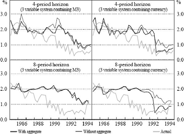
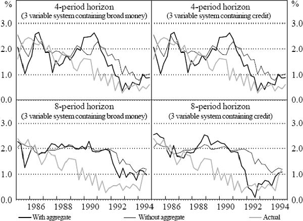
The detailed out-of-sample forecasting results for systems containing the aggregates are presented in Appendix B, Tables B1 to B8. All forecast statistics for the aggregates are listed in these tables in the Appendix. A summary of the results is presented below in Tables 3 and 4. For the inflation forecasts, we also present Figures (6 and 7) of the forecasts for the 4 and 8-period horizons for models with each aggregate to identify whether any improvement in the forecasting accuracy is consistent over the entire forecast sample.
| Model(a) | Ratio statistic |
|---|---|
| 2VM3 | Slight improvement over steps 2–6(b) |
| 3VM3 | Slight improvement over steps 5–8 |
| 4VM3 | Slight improvement at steps 7 and 8 |
| 5VM3 | Worse over 7 of 8 steps |
| 2VCU | Uniformly worse |
| 3VCU | Uniformly worse |
| 4VCU | Uniformly worse |
| 5VCU | Uniformly worse |
| 2VBM | Uniformly worse |
| 3VBM | Worse over 6 of 8 steps |
| 4VBM | Worse over 7 of 8 steps |
| 5VBM | Slight improvement at steps 6 and 8 Notable improvement at step 5(c) |
| 2VCR | Uniformly worse |
| 3VCR | Uniformly worse |
| 4VCR | Uniformly worse |
| 5VCR | Uniformly worse |
Notes: (a) The prefix in this column refers to the number of
variables in the system eg 2VM3 is the two-variable system containing M3. |
|
| Model(a) | Ratio statistic |
|---|---|
| 2VM3 | Slight improvement over steps 4–8(b) |
| 3VM3 | Uniformly worse |
| 4VM3 | Uniformly worse |
| 5VM3 | Uniformly worse |
| 2VCU | Notable improvement over steps 4–8 (c) |
| 3VCU | Slight improvement over steps 5–8 |
| 4VCU | Slight improvement over steps 5–8 |
| 5VCU | Uniformly worse |
| 2VBM | Notable improvement over steps 5–8 |
| 3VBM | Slight improvement over steps 5–8 |
| 4VBM | Slight improvement over steps 6–8 |
| 5VBM | Uniformly worse |
| 2VCR | Uniform notable improvement |
| 3VCR | Uniform improvement. Notable improvement at steps 6–8 |
| 4VCR | Slight improvement over steps 2,4 and 5 Notable improvement at steps 6–8 |
| 5VCR | Slight improvement over steps 6–8 |
Notes: (a) The prefix in this column refers to the number of
variables in the system eg 2VM3 is the two-variable system containing M3. |
|


As was the case for the in-sample tests, the results are mixed. There appears little evidence that the inclusion of any of the financial aggregates improves the out-of-sample forecasts of real GDP growth. For inflation forecasting, the results appear somewhat more positive, although they do not seem to be robust over the entire sample. Currency shows some contribution to improving the forecasting accuracy for inflation relative to the model without currency, consistent with some of the in-sample evidence. Broad money also shows some improvement in the forecasts of inflation in the latter quarters of the forecast horizon, but only in the two-variable VAR is there evidence of notable improvement. Inclusion of credit in the VAR improves forecast accuracy for inflation towards the end of the forecast horizon, but the improvement is strongest in the two and three-variable VARs. M3 appears to make no contribution to out-of-sample forecasting performance.
To keep these results in perspective, it should be noted that none of the models yields particularly good out-of-sample inflation forecasts. Figures 6 and 7 illustrate that the forecasts from both VAR models generally overpredict inflation over the forecast sample. In cases where some forecast improvements do occur, Figures 6 and 7 illustrate that the improvement to the forecast of inflation is confined to the latter part of the forecast sample. As discussed above in the data section, the forecast improvement may be reflecting the dramatic decline of the growth of the aggregates along with inflation after 1990, and does not appear to be a general result applicable to the sample as a whole.
Footnotes
The data series we employ have been revised thus reflecting information unavailable at the time of the forecast, so the tests are not purely ‘real time’ forecasting experiments. [19]
It is notable that errors in the forecasts become compounded in the dynamic setting, but it remains the most realistic setting to evaluate forecasts. [20]
The ratios of the root mean squared error (RMSE) is comparable to the Theil-U statistic used in forecast evaluation that compares a forecast RMSE to that of a random walk forecast. In our case, if the financial aggregates add no value to the forecast, the two VAR model alternatives should have comparable RMSE for forecasting output growth and inflation. In that case, the ratio values should be close to one. [21]