RDP 9606: The Information Content of Financial Aggregates in Australia 4. Empirical Methods
November 1996
- Download the Paper 279KB
4.1 In-Sample Tests – Overview
The information content of the financial aggregates is initially assessed by examining their forecasting power for subsequent observations of output growth and inflation on an in-sample basis. The ordering of tests is from the simplest models to the most complex, so as to ascertain whether money correlations are robust by examining systems with an increased number of variables. The models are specified in first difference form due to test statistics that suggest nonstationarity of the data in log-level form. We note, however, that the tests have low power, and as a result, we also estimate systems in log-levels (except for the interest rate).[10] Each VAR is estimated with 4 lags of each variable in the system. The structure is outlined below:
| xt = A(L) xt−1 + εt | |
| where | xt is the vector of endogenous variables. |
| εt is the vector of error terms. |
A is a series of square matrices representing correlations among endogenous variables, and L is the lag operator.
The methodology involves examining F-tests, block exogeneity tests, and variance decompositions for each of the systems under consideration.[11] The F-tests measure whether money is significant for predicting real GDP and the CPI in the single reduced form equation for the respective variables. F-tests are examined for the two, three, four and five-variable systems containing the respective financial aggregates. The basic two-variable system contains the growth rate of the financial aggregate and inflation or the growth rate of output. The three-variable system contains the growth rate in money, real output growth, and inflation. The four-variable system adds the differenced interest rate while the five-variable system adds also the differenced exchange rate.
In bi-variate VARs, the F-test is equivalent to a Granger causality test. In the larger VAR systems, the F-tests are insufficient for determining Granger causality because the restrictions test only the direct effect of money in single equations of inflation and output growth. For the VAR systems of three or more variables, we therefore test whether the system is block exogenous to the movements in the financial aggregates. These tests are interpreted as detecting whether the relevant financial aggregate is important to the system as a whole. We follow up on these results by employing a standard tool of VAR analysis, the variance decomposition, to uncover their quantitative importance in predicting output and inflation.[12]
The variance decompositions measure the percentage of forecast error variance in real output growth and inflation that can be attributed to innovations in the particular financial aggregate under examination. The extraction of variance decompositions from a VAR typically requires orthogonalisation of the errors from the reduced-form equations. We orthogonalise the shocks to the four-variable VAR system using a Choleski decomposition, which implies a recursive structural ordering for the variables.[13]
Using the Choleski decomposition from the reduced form errors, orthogonal innovations can be obtained in the following way, which is equivalent to running OLS on the reduced form errors:
| εt1 = υt1 |
| εt2 = R1 εt1 + υt2 |
| εt3 = R2 εt2 + R1 εt1 + υt3 |
| εt4 = R3 εt3 + R2 εt2 + R1 εt1 + υt4 |
where:
| the Ri's are OLS regression coefficients |
| εti are the reduced-form error terms and |
| υti are the orthogonal errors. |
Orthogonal errors, υt, are required in order to generate variance decomposition evidence.
Evidence from variance decompositions investigates the explanatory power of financial aggregates for forecasting real output and inflation. The Choleski factorisation orthogonalises the variance-covariance matrix so that the Choleski factor is lower triangular with positive elements on the diagonal (positive variance). This is what imposes the recursive ordering on the variance decomposition results.
Variance decomposition results can be sensitive to both the ordering imposed on the system as well as the data sample. For our variance decomposition results, we experimented with three estimated VAR models. The base specification estimates a VAR over the full sample period with the following ordering (recursive structure): change in the interest rate, monetary aggregate growth, inflation, and real output growth.[14]
Placing the financial aggregate second in the ordering allows innovations in the equation for financial aggregates to affect contemporaneously inflation and real output growth. The motivation for this ordering is to test the contribution of the financial aggregate measure to forecasting output and inflation in a favourable specification. By placing the growth rate in the aggregate ahead of output growth and inflation in the ordering, we increase the chances of finding results that show orthogonalized innovations in financial aggregates influencing the subsequent behaviour of output growth and inflation. In such an ordering, the innovation associated with the financial aggregate appears in the equations for output growth and inflation in the system, whereas innovations to output and inflation do not appear in the equation for the financial aggregate. This is a strong identification restriction. The second specification generates variance decomposition results from an abbreviated sample that ends in 1988:Q4 using the ordering from the base specification. The third specification places the financial aggregate last in the ordering and estimates the VAR over the full-sample. By placing the financial aggregate last in this case, we restrict the contemporaneous impact of innovations to the financial aggregates on inflation and output growth to be zero. The results from the final ordering highlight the importance of the contemporaneous correlations on the subsequent results.
Attention in the discussion below is focused on the four-variable VAR results, although initial results using a five-variable VAR are generally consistent with these.[15]
4.2 In-Sample Results
We begin by generating F-test p-values from a sequence of data samples starting from the shortest sample 1976:Q4 to 1984:Q1. The procedure then adds one more observation and generates the F-test and the associated p-value, continuing this process until the end of the sample [1995:Q3]. A similar procedure is followed for block exogeneity restrictions in the larger systems.
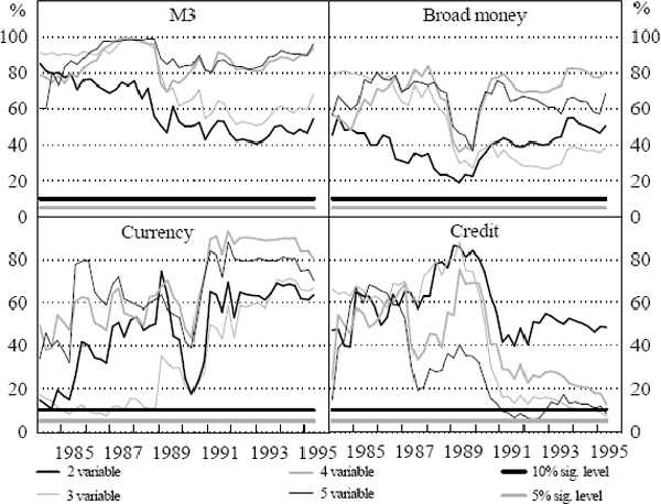
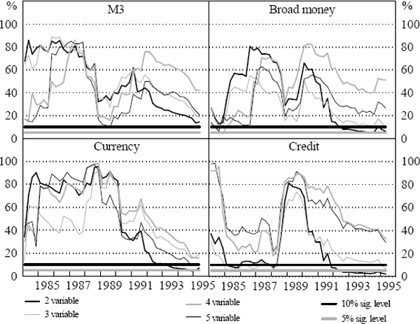
The F-test results for systems containing the respective aggregates are shown in Figures 3 and 4. The figures summarise the results from the tests of the joint significance of four lags of money in the output growth and inflation equations respectively. The F-tests have been done for each of the output growth and inflation equations in the two, three, four and five-variable systems. For each aggregate, there is a line that reflects the p-value from the F-test of the exclusion restriction, one line for each of the four estimated systems. The solid black horizontal line in each panel indicates the 10 per cent significance level while the solid grey horizontal line indicates the 5 per cent significance level. When the line reflecting the p-value of the restrictions crosses the solid horizontal lines, it implies a rejection of the restriction at the specified significance level.


The F-test results for the output growth equations indicate that M3, currency and broad money are not significant for predicting real GDP. In contrast, credit appears significant in some instances in the three and five-variable systems for predicting real output growth.
For inflation equations, the F-tests indicate that M3 is not significant for predicting inflation in any of the VAR systems. Results for the other aggregates are mixed, with significant predictive power in a subset of cases. Currency appears significant for predicting inflation in the two and five-variable systems for samples ending after 1993:Q2. Broad money and credit appear important after 1992 in the two and possibly three-variable cases. However, these results are not robust to the addition of interest rate and exchange rate variables, so we do not give them much credence.[16]
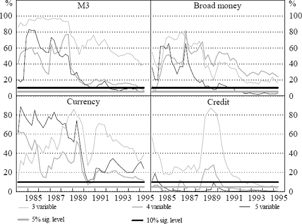
On a similar basis, we present p-value charts for block exogeneity tests for the financial aggregates for the three, four, and five-variable VAR systems in Figure 5. The results suggest that M3 is important in the four and five-variable systems towards the end of the sample. In contrast to the M3 results, the test results for currency indicate that it is not statistically significant for any of the systems over any portion of the sample period. Broad money appears significant only in the five-variable system after 1991. The most consistently significant variable is credit, which appears statistically significant in the three, four and five-variable systems after 1992. It is notable, however, that for the credit aggregate the p-value rises dramatically for the three and four-variable systems between 1988 and 1990, perhaps reflecting instability in the relationship between credit and policy variables during the asset price volatility at that time.

These block exogeneity tests are not conclusive evidence that financial aggregates are unimportant for output growth and inflation, because they ignore the possibility that there are important contemporaneous correlations among the data. We generate variance decompositions to explore this issue further.
The results for the three specifications of the variance decompositions are listed in Tables 1 and 2, which also present 90 per cent confidence bounds on these variance decompositions to help infer the statistical importance of the results.[17] The bounds provide one method to infer the statistical importance of innovations associated with a financial aggregate in a variance decomposition.
| Aggregate in system | Variance of: |
Forecast horizon | Per cent of forecast innovations explained by innovations in the financial aggregate(a) | ||
|---|---|---|---|---|---|
| Initial ordering 1977:Q4–1995:Q3 |
Initial ordering 1977:Q4–1988:Q4 |
Ordering with M after P,Y 1977:Q4–1995:Q3 |
|||
| M3 | Inflation |
6 |
3.7 (1.7, 16.1) |
7.1 (4.2, 35.7) |
3.3 (1.3, 13.3) |
| 12 |
5.4 (2.0, 25.9) |
7.4 (5.5, 45.0) |
3.0 (1.5, 19.1) |
||
| Output growth |
6 |
14.1 (6.2, 30.4) |
8.8 (5.2, 35.2) |
3.4 (1.6, 14.6) |
|
| 12 |
15.4 (6.9, 32.4) |
8.6 (7.3, 40.7) |
4.6 (2.3, 17.7) |
||
| CU | Inflation |
6 |
13.2 (3.7, 29.0) |
4.7 (2.4, 20.8) |
13.4 (3.5, 26.4) |
| 12 |
18.2 (5.3, 35.5) |
5.4 (2.9, 23.9) |
15.7 (4.1, 29.0) |
||
| Output growth |
6 |
6.2 (2.4, 19.0) |
6.0 (3.1, 21.7) |
1.6 (0.9, 10.5) |
|
| 12 |
7.1 (3.2, 20.7) |
5.9 (4.2, 23.7) |
2.2 (1.4, 12.2) |
||
Note: (a) Each variance decomposition represents the per cent of forecast error variance explained by the innovation associated with the variable at the top of the column. The percentile bounds are in parentheses. |
|||||
| Aggregate in system | Variance of: |
Forecast horizon | Per cent of forecast innovations explained by innovations in the financial aggregate(a) | ||
|---|---|---|---|---|---|
| Initial ordering 1977:Q4–1995:Q3 |
Initial ordering 1977:Q4–1988:Q4 |
Ordering with M after P,Y 1977:Q4–1995:Q3 |
|||
| BM | Inflation |
6 |
15.0 (3.6, 33.4) |
12.1 (4.2, 34.1) |
6.6 (2.0, 19.6) |
| 12 |
30.3 (8.4, 51.1) |
15.4 (5.6, 38.0) |
14.9 (2.8, 33.5) |
||
| Output growth |
6 |
17.4 (7.5, 32.7) |
6.8 (4.1, 26.9) |
6.0 (2.3, 17.3) |
|
| 12 |
19.0 (9.9, 35.3) |
8.1 (6.2, 34.4) |
7.9 (3.3, 21.6) |
||
| CR | Inflation |
6 |
16.3 (4.9, 33.5) |
5.7 (2.2, 20.7) |
8.2 (2.2, 19.1) |
| 12 |
40.0 (17.4, 55.1) |
8.8 (3.2, 25.6) |
16.9 (6.2, 28.8) |
||
| Output growth |
6 |
24.0 (11.4, 38.6) |
7.3 (3.4, 22.0) |
8.7 (3.0, 19.2) |
|
| 12 |
23.6 (11.6, 37.8) |
8.6 (4.5, 24.0) |
9.0 (3.6, 19.5) |
||
Note: (a) Each variance decomposition represents the per cent of forecast error variance explained by the innovation associated with the variable at the top of the column. The percentile bounds are in parentheses. |
|||||
Runkle (1987) argues that variance decomposition results should be considered important if the lower bound is above 10 per cent. We use this general suggestion as a guide to the importance of the variance decomposition. Employing this criterion, there is no aggregate that explains an important proportion of the forecast error variance of either output growth or inflation in all of the three specifications of the VAR. For example, over the 12-quarter horizon, credit explains about 40 per cent of subsequent fluctuations of inflation (with a lower bound of approximately 17 per cent) using the initial ordering over the full sample. In the other two specifications, the explanatory power of the credit innovation at the 12-quarter horizon greatly diminishes, to the extent that it appears no longer important, that is, the lower bounds fell below 10 per cent. There is a similar lack of robustness whenever a significant result is found. In contrast to previous studies, there appears to be no explanatory power for M3 as an inflation predictor in any specification.[18]
Footnotes
Results are available on request from the authors. Use of levels rather than differences affects some of the in-sample inferences but has little effect on the out-of sample results. [10]
Both F-test and block exogeneity tests employ the reduced form of the VAR. In contrast, the variance decomposition results require orthogonalization of the reduced-form errors. [11]
Variance decompositions reveal the proportion of forecast variance explained by innovations associated with it or another variable. See Hamilton (1994). [12]
We adopt an agnostic view of the ordering as ‘structure’, choosing this method because it provides directly interpretable results for examining whether a monetary aggregate contributes forecasting power for real output and inflation. [13]
We justify this formulation as the base specification by suggesting that monthly numbers for the aggregates are available before the release of inflation and output measures. The interest rate variable is observable more frequently than financial aggregates and is placed before the aggregate in the ordering using the same temporal justification as above. [14]
In addition, the four-variable VAR does not involve the difficulty of forecasting the change in the exchange rate. Out-of-sample results suggest that the inclusion of the exchange rate worsens out-of-sample forecast performance of the VAR as well. [15]
The sum of the coefficients on the four lags of the financial aggregate variables in the output equations estimated over the full sample were as follows: −.0384 for M3, .0504 for BM, .2937 for credit, and .0552 for currency. Similarly for the inflation equations, the sums were: −3.507E-3 for M3, .0750 for BM, .1181 for credit and .1532 for currency. None of the coefficient sums were statistically different from zero at the 10 per cent level in the four-variable specification over the full sample. [16]
The 90 per cent probability bands are calculated for each specification of the variance decompositions using Monte Carlo integration techniques similar to those described in the RATS 4.0 manual. We generate 1,000 draws of the variance-covariance matrix, generate associated variance decompositions, and choose the 5th and 95th percentile observations. These extreme observations provide the error bands. Details of the procedures are available from the authors upon request. [17]
We note that these negative results contrast with results in Orden and Fisher (1993) in which M3 had significant impact on the price level. This may be due to the difference in the data sample as well as their use of an error-correction specification. [18]