RDP 9507: Macroeconomic Policies and Growth Appendix a: Influences on Growth
October 1995
- Download the Paper 184KB
A1. The Persistence of Growth Rates and the Determinants of Growth
As briefly discussed in the text, while levels of output have a high degree of persistence, for most countries, growth is not very persistent. The correlation between average growth rates in the 1960s and in the 1970s is as low as 0.15 for 89 non-oil countries and only slightly higher (0.3) when the same calculation is done for the 1970s and 1980s (Easterly et al. 1993). By contrast, country characteristics, including many policy related variables used in most cross -country regressions, are highly persistent.
We have explored this problem further for the OECD countries (excluding Iceland and Turkey) in Table A1 by regressing average growth for 5-year periods over subsequent 5-year periods. Panel (a) of the table shows that out of 21 correlation coefficients only 4 are significant, with the highest being the one for the two sub-periods of the 1960s. By contrast, as panels (b) to (d) show, inflation as well as general government deficits and investment (both as ratios to GDP) exhibit much more persistence than growth. For investment, even ratios 30 years apart yield a coefficient of almost 0.5. For inflation, the effect of the two oil shocks is clearly evident while the degree of persistence strengthens considerably for the more recent years when inflation declined. Budget deficits, on the other hand, have become less persistent in recent years, probably reflecting countries' differential success in consolidating their fiscal positions.
| 1965/70 | 1970/75 | 1975/80 | 1980/85 | 1985/90 | 1990/95 | |
|---|---|---|---|---|---|---|
| (a) GDP growth | ||||||
| 1960/65 | .74* | .30 | .19 | .02 | .14 | .26 |
| 1965/70 | .43 | .52* | .12 | .50* | .08 | |
| 1970/75 | .28 | .48* | .39 | .28 | ||
| 1975/80 | .01 | .31 | .19 | |||
| 1980/85 | .10 | .38 | ||||
| 1985/90 | .20 | |||||
| (b) Inflation | ||||||
| 1960/65 | .50* | .45** | .01 | .15 | .31 | .12 |
| 1965/70 | .31 | .06 | .23 | .31 | .43 | |
| 1970/75 | .69* | .50* | .35 | .32 | ||
| 1975/80 | .85* | .85* | .52* | |||
| 1980/85 | .87* | .72* | ||||
| 1985/90 | .82* | |||||
| (c) General government deficit/GDP | ||||||
| 1960/65 | .83* | .73* | .71* | .60* | .46 | .01 |
| 1965/70 | .83* | .75* | .48** | .50* | .01 | |
| 1970/75 | .78* | .56* | .41 | .03 | ||
| 1975/80 | .59* | .35 | .00 | |||
| 1980/85 | .56* | .18 | ||||
| 1985/90 | .38 | |||||
| 1960 | 1970 | 1980 | 1990 | |||
| (d) Investment/GDP | ||||||
| 1960 | .78* | .57* | .48** | |||
| 1970 | .73* | .66* | ||||
| 1980 | .64* | |||||
|
Note: The numbers shown in panels (a) and (b) are correlation coefficients between average rates of respectively real GDP growth and inflation for the five -year periods in the first column and the subsequent five -year periods given in the first row. Similarly the numbers in panels (c) and (d) are correlation coefficients between respectively government deficit and investment/GDP ratios for the periods or years shown in the first column and the periods or years given in the first row. * and ** indicate respectively 99 and 95 per cent levels of significance. |
||||||
What is the relevance of these results for the link between policies and growth? First, country characteristics are not the only determinants of growth; as Easterly et al. conclude, a substantial part of the variation in growth arises from shocks, in particular terms-of-trade shocks. Second, one interpretation of the results is that country characteristics mainly serve to explain relative per capita income levels while growth rates are more dependent on shocks, and are therefore more variable. Nonetheless, policies can still have a significant influence on growth, especially when countries are far from their steady-state income levels. Third, while shocks are important in explaining growth, policy reactions to the shocks influence how growth is affected. For instance, when comparing the coefficients in Table A1 for the two oil shocks, it is noticeable that following the first oil shock (1965/70 to 1970/75) the correlation for GDP growth remained at a relatively high 0.43 while for inflation the correlation fell to 0.31. By contrast, between 1975/80 and 1980/85 the correlation for GDP growth declined to only 0.01; inflation, on the other hand, remained highly persistent because most countries tightened monetary policy to prevent the second oil shock from pushing up inflation.
A2. Growth and Balance of Payments
The McCombie and Thirlwall model
To derive their balance-of-payments consistent growth rate, McCombie and Thirlwall (1994) [MT] start from the balance-of-payments identity:

where: Pd is export prices in domestic currency;
Pf is import prices in foreign currency;
X is exports of goods and services (in volumes);
M is imports of goods and services (in volumes);
E is the exchange rate (measured as domestic currency per unit of foreign currency); and
F is the capital account balance.
No distinction is made between export prices and domestic prices, which implies that the real effective exchange rate is identical to the terms of trade.
Export and import volumes depend on income and relative prices as follows:
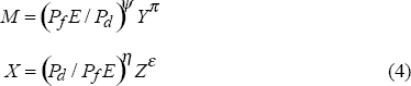
where: ψ = demand elasticity of imports with respect to relative price of imports;
η = demand elasticity of exports with respect to relative price of exports;
π = elasticity of imports with respect to domestic income (Y); and
ε = elasticity of exports with respect to foreign income (Z).
Taking rates of change, denoted by small letters, (4) becomes:
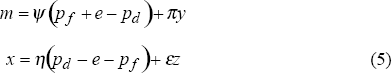
Similarly, equation (3) can be rewritten in rates of change:

where θ denotes the proportion of import expenditure met by export earnings. Then inserting (5) into (6), the balance-of-payments constrained growth rate can be written as:

where the first term on the right-hand side measures the trade volume effects of relative price changes and will be positive for a real depreciation (or terms-of-trade deterioration); the second term the income effect of terms-of-trade changes; the third term the effect of export growth; and the last term the effect of capital flows (measured in constant prices) which is positive in case of inflows. The sum of the four terms determines total revenue available for expanding imports and the corresponding growth of income is then derived by dividing by the income elasticity of imports.
To provide estimates of y* for Australia within the MT framework, two specific problems need to be addressed. First, how should capital inflows be defined and measured? One possibility is to include only those flows (for instance, foreign direct investment, equity portfolio inflows and long-term debt inflows contracted by the private sector) that are mainly attracted by prospective returns in the Australian private economy.[28] Alternatively, one can ignore capital inflows in the calculation of y* and leave them for an ex post evaluation in the event that actual output growth deviates from y*. A second issue is the treatment of net income and transfers, which are not included in MT's measure of revenue available for imports but would significantly affect y* if they do not remain constant. To generate our results, we include changes in capital inflows only as a memorandum item, and subtract the growth of net income payments to abroad from the growth of export earnings, with a weight corresponding to their share of total export revenue. With these assumptions, Table A2 shows our estimates, using average figures for 1959/60–1993/94 and the shorter period 1972/73–1989/90.
| Variables | Actual and estimated values: | |
|---|---|---|
| 1959/60–1993/94 | 1972/73–1989/90 | |
| Growth in net income payments to abroad | 6.5 | 8.3 |
| Change in the terms of trade | −0.5 | 0.6 |
| Growth in export volumes | 6.0 | 4.5 |
| Adjusted export growth(a) | 4.50–5.00 | 3.25–4.00 |
| Balance-of-payments constrained GDP growth (b) | 2.75–3.05 | 2.00–2.45 |
| Actual GDP growth | 3.7 | 3.1 |
| Change in capital inflows: as per cent of GDP | 1.0 | 5.1 |
|
Notes: (a) Obtained from equation (5) by subtracting the weighted growth of net
income payments (weight = the share of net income in total export revenue) and
the combined effect on income and trade volumes of terms of trade changes,
allowing for two extreme cases: θη+ ψ + 1 = 0 (i.e. no adjustment
to export growth) and θη + ψ = 0 (i.e. export growth adjusted for
the full terms-of-trade change). |
||
The implications of rising external liabilities
To derive the results in the text, we use the following empirical ingredients. First, the Blundell-Wignall et al. (1993) equation for the Australian real exchange rate, when re-estimated over the period 1984:1 to 1994:4, implies that a one percentage point rise in the ratio of net external liabilities to GDP is associated with a real depreciation of 0.5 per cent.
Second, the relationship between net external liabilities (NEL) in years t and t+1 and the current account deficit (CAD) in year t is given by NELt+1=NELt+CADt. Dividing throughout by GDP and letting lower-case letters denote ratios to GDP gives:

where g is nominal GDP growth per annum. Assuming g = 0.06, a current account deficit of 4.5 per cent of GDP (average for the last ten years) and a net external liabilities to GDP ratio of 45 per cent (the current value) implies that the net external liabilities to GDP ratio is rising by 1.7 percentage points per annum, leading to an average annual real exchange rate depreciation of 0.5 X l.7 = 0.85 per cent.[29]
Third, to estimate the inflationary impact of this real exchange rate depreciation, we rely on the price equation in Wilkinson and Lam (1995) which explains domestic prices in the long-run by unit labour costs and import prices, with coefficients 0.7 and 0.3 respectively. In the long run, a 1 percent nominal depreciation therefore raises domestic prices by 0.3 per cent and hence translates into a real depreciation of 1 − 0.3 = 0.7 per cent. It follows that a real depreciation of 0.85 per cent per annum generates a rise in domestic prices of 0.3 × 0.85 / 0.7 = 0.36 per cent per annum.
To completely offset the domestic price effect of the real depreciation, real unit labour costs must fall by 0.3 × 0.85 / 0.7 = 0.36 per cent per annum. With no explicit mechanism to reduce real unit labour costs, this outcome can only be achieved by reducing the level of real output. To derive the required reduction, we use the sacrifice ratio of 2.5 (Stevens 1992). To prevent the real depreciation and the rise in import prices from pushing up the domestic inflation rate, actual output must be reduced on average by about 0.9 per cent (0.36 × 2.5).
A3. Inflation and Growth
The LR base regression applied to the 22 low inflation OECD countries is:

( = 0.61,
estimation period 1960–89, absolute value of White robust t-statistics in parentheses),
while the LZ base regression applied to the 22 low inflation OECD countries is:
= 0.61,
estimation period 1960–89, absolute value of White robust t-statistics in parentheses),
while the LZ base regression applied to the 22 low inflation OECD countries is:

( = 0.57,
estimation period 1960–89, absolute value of White robust t-statistics in parentheses).
The variables are average per capita real GDP growth in per cent per annum (Δq), per capita real GDP in 1960 (RGDP60), average annual rate of population growth (GPO), initial secondary school enrolment rate (SEC), average investment share of GDP (INV) and the average number of revolutions and coups per year (REVC). LRGDP60 and LSEC are log(RGDP60) and log(SEC).
For the set of LR regressions, the Z-variables are: government consumption share of GDP (GOV), export share of GDP (X), the average number of revolutions and coups per year (REVC), and the ratio of liquid liabilities to GDP (LLY), while for the set of LZ regressions, the Z-variables are: the government fiscal surplus ratio to GDP (SURY), the ratio of total trade to GDP (TRD), LLY and the black-market exchange rate premium (BMP).[30]
Both the LR and LZ base regressions contain statistically insignificant explanatory variables when estimated for the 22 low inflation OECD countries (see above). We include these variables in the analysis reported in the text to reproduce the LR-LZ approach as closely as possible. Nevertheless, to establish that our conclusions about the correlation between inflation and growth are robust to the exclusion of these variables, we repeat the analysis for the whole estimation period 1960–89 and for the sub-period 1960–73, excluding from each base regression any variable with an absolute t-statistic less than 1.5. This implies that, for the LR whole estimation period regression, GPO and SEC are excluded, for the LZ whole estimation period regression, LSEC is excluded, for the LR 1960–73 regression, SEC is excluded, while for the LZ 1960–73 regression, LSEC is excluded.
These modified LR and LZ regressions generate the following results. The coefficient on average inflation in all 30 regressions estimated over 1960–89 is negative with point estimates ranging from −0.11 to −0.20, mostly significant at 5 per cent. For the 15 LR and 8 LZ regressions estimated over the sub-period 1960–73, the coefficient on average inflation is negative in 20 (out of 23) regressions with point estimates ranging from −0.09 to +0.01 but always insignificant at a 10 per cent level. We infer from this exercise that the conclusions drawn in the text about the inflation-growth relationship are robust to the exclusion of insignificant explanatory variables from the LR and LZ base regressions.
We also looked for any systematic non-linearity in the relationship between growth and inflation for our sample, and sub-samples, of OECD countries. To do so, we added the square of average inflation, PI2, to each regression in our original analysis. No systematic results emerged from this exercise, with both the size and sign of the coefficients on PI and PI2 often changing from one regression to the next.
For completeness, we also report results adding average inflation (PI) to the LR and LZ base regressions when the sample includes all 24 OECD countries. The LR regression is then:

( = 0.58,
estimation period 1960–89, absolute value of White robust t-statistics in parentheses),
while the LZ regression is:

( = 0.50 ,
estimation period 1960–89, absolute value of White robust t-statistics in parentheses).
Footnotes
As noted in IMF (1995), countries with abundant natural resources tend to have large and sustained capital inflows. Higher labour-force growth should have a similar effect. [28]
The current nel value of 45 per cent is calculated by cumulating current account deficits since 1970. This is the relevant measure for our purposes since we use the Blundell-Wignall et al. estimate of the sensitivity of the real exchange rate to changes in nel. Note, in passing, that the effect of a given current account deficit on the change in nel is inversely related to the actual size of nel. On the other hand, the sensitivity of the current external imbalance to changes in foreign interest rates increases in proportion to nel. Both relations are relevant to the notion of a balance of payments constraint, but will not be discussed further. [29]
These Z-variables correspond closely to those used by LR and LZ. We added LLY (one of the LZ Z-variables) to the list of Z-variables used by LR to generate more regressions. For the LZ sub-sample regressions, we used GOV instead of SURY, but lacked data on BMP and so were limited to eight regressions for each sub-sample. [30]