RDP 9306: Inventories and the Business Cycle 4. Demand, Costs and Inventories: Evidence from Survey Data
June 1993
- Abstract
- Download the Paper 113KB
One way to overcome the problems induced by estimating expectations from an econometric model is to use actual surveys of firms' expectations. Since 1961 the quarterly ACCI/Westpac Survey of Industrial Trends has asked over 200 firms a number of questions concerning their actual and expected changes in production, stocks, orders, prices and costs etc. Specifically, the survey asks the following question for a range of variables:
excluding normal seasonal changes, what has been your company's experience over the past three months and what changes do you expect during the next three months?
Companies are asked to answer increase, decrease or remain the same. Our interest is in the answers to the questions regarding actual and expected changes in costs, new orders, stocks of finished goods and stocks of raw materials. Unfortunately, the survey does not publish the responses of individual firms. It does, however, publish the percentage of firms that answer ‘increase’, ‘decrease’ and ‘remain the same’ to each question.
Since the survey asks whether the firm expects an increase in the relevant variables there is no need to use a model to estimate the expected changes and innovations. They are directly observable. For example, the innovation in demand at time t can be calculated by taking the difference between the percentage of firms that actually report an increase in new orders at time t and the percentage that, at time t-1, thought new orders would increase. If the percentage of firms that report an increase in demand exceeds the percentage that thought demand would increase, a positive shock to demand can be said to have occurred. Similar calculations can be performed to obtain the shocks to inventories of both raw materials and finished goods.
In addition to using the difference between the percentage of firms that experience and expect an increase in orders, stocks etc., we also use the difference in the percentage that actually report a decline in orders, stocks etc., and the percentage that expected a decline. Finally, we also use the net balance figures. The actual (expected) net balance is the difference in the percentage of firms that report (expect) an increase and the percentage that report (expect) a decrease. All three measures of the shocks should provide similar results.
Graph 4 shows the calculated shocks to both orders and the stocks of finished goods calculated using the ‘net balance’ figures. There are two interesting points to note. First, the shocks to orders are typically unfavourable shocks. That is, the number of firms that actually report an increase in orders is generally less than the number that predicted an increase in orders. Over the entire sample period, the average ‘shock’ is −8.5 per cent. If the forecasts are unbiased this average shock should be insignificantly different from zero. A test of the unbiased hypothesis is, however, overwhelmingly rejected.[11] Firms appear to be consistently excessively optimistic about their new orders. This optimism is also reflected in the fact that stocks of finished goods typically increase by more than was expected. The average expectation error is +7.9 per cent. Again, this is significantly different from zero. It is unclear why these persistent errors exist.[12]
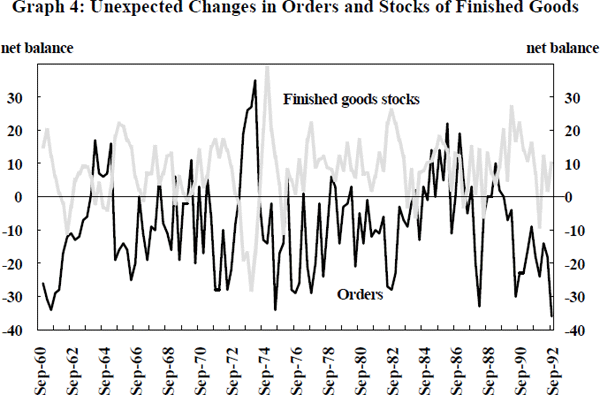
More interesting for the question at hand is the apparent negative correlation between the shocks to demand and inventories. A number of episodes clearly stand out. The unexpected declines in orders in the second half of 1974, 1982 and 1990 were all associated with an unexpected increase in inventories. Similarly, in the 1960s unexpected increases in inventories occur when demand is unexpectedly low. In Table 5 we present the correlation coefficients between the forecast errors for orders and the forecast errors for inventories of both finished goods and raw materials. Correlations are calculated using the ‘up’, ‘down’ and ‘net balance’ figures. They are calculated using data from the entire period as well as data for each half of the sample.
| Sample Period | |||
|---|---|---|---|
| Inventories Of: | 60:3 – 92:3 | 60:3 – 76:3 | 76:4 – 92:3 |
| Finished Goods | |||
| • Up | −0.30** | −0.48** | −0.03 |
| • Down | −0.30** | −0.49** | −0.06 |
| • Net balance | −0.40** | −0.57** | −0.15 |
| Raw Materials | |||
| • Up | 0.11 | −0.01 | 0.27* |
| • Down | 0.05 | −0.17 | 0.29* |
| • Net balance | 0.04 | −0.12 | 0.23 |
| Notes. 1. * (**) indicates that the correlation coefficient is statistically different from zero at the 5 (1) percent level. 2. The correlations for ‘up’ are the correlations between the forecast errors calculated using only the ‘increase’ responses for both orders and inventories. The ‘down’ correlations use only the ‘decrease’ responses. |
|||
Using data over the entire period we find a strong negative and statistically significant relationship between shocks to orders and shocks to inventories of final goods. Over the full sample period the correlation coefficient (using the net balance figures) is −0.40 which is significantly different from zero at conventional significance levels. In contrast, the correlation using the stocks of raw materials is small and is insignificantly different from zero. Similar results are obtained using both the ‘up’ and ‘down’ responses.[13] These results suggest that when demand for a firm's product is unexpectedly low, its stocks of finished goods are unexpectedly high, but that there is no unexpected change in the firm's stocks of raw materials. This indicates that when faced with an adverse shock to demand, firms do not reduce their production immediately but instead build up their stocks of finished goods. This is consistent with inventories of finished goods being used, in the first instance, as a buffer stock to demand shocks. Given that production and inventory accumulation initially continue in the face of the demand shock, it is hardly surprising that there is no immediate unexpected accumulation of raw materials stocks.
The results in Table 5 also suggest that there has been a change over time in the relationship between innovations in orders and innovations in inventories of finished goods. Over the first half of the sample period the correlation coefficient between demand forecast errors and finished goods inventory forecast errors is −0.57 while over the second half of the sample period the coefficient is just −0.15. The hypothesis that the coefficients are the same can be rejected at the 5 per cent level.
The above results for the stocks of finished goods stand in contrast to those reported in Table 4. Unlike the macro-results, the results from the survey suggest that unexpected falls in demand are reflected in unexpected increases in stocks. The difference in results may reflect the inability of the innovations from the ARMA models of inventories and output to accurately represent the true innovations. The forecasts from the ARMA models only use information contained in past values and the error terms. In contrast, while it is unclear to the econometrician what information goes into generating the firms' forecasts, these forecasts should be based on a much wider information set than that available to the time-series econometrician.[14] While, the forecasts from the ARMA models may be unbiased, the measured innovations may not be the true innovations. Suppose that the innovations from the ARMA models (εt and μt) each consist of two components and that each of these components has a zero mean. That is:


and E(ϕ)=E(φ)=E(ν)=E(ζ)=0. Let the first component in each of the ARMA innovations represent the true innovation and the second component the error made by the econometrician through not being able to observe the complete information set. Assume that the errors induced by incomplete information are uncorrelated with the true innovations (E(ϕφ)=E(νζ)=E(ϕν)=E(ϕζ)=0). Given this assumption, the correlation between the two ARMA innovations is given by:

The results from the survey data suggest that the true innovations are negatively correlated; that is, E(ϕν) is less than zero. However, the results in Table 4 show that E(εμ) is approximately zero. This implies that E(φζ) is positive. Given that the same unobservable information is likely to be used in forecasting both demand and inventories it is not surprising that the errors induced by incomplete information are correlated. The fact that they are positively correlated suggests that when information, not included in the ARIMA model, leads firms to expect demand to be low, this same information leads firms to expect that inventories will also be low. This issue is examined in more detail below. More generally, the conflicting results from the aggregate and survey data suggest a general warning concerning the ability of ARMA models to generate true economic innovations.
The above results from the survey data suggest that firms have used their stocks of finished goods as a buffer against shocks to demand. The above reconciliation of the survey and the macro-data results also suggest that expected increases in demand are associated with expected increases in stocks. The model presented in Section 2 suggested such a positive correlation provided that changes in demand had reasonable degree of persistence. A negative correlation between the expected changes in demand and inventories is only predicted if production smoothing is extremely important and changes in demand are viewed as shortlived. We now turn to an examination of the relationship between expected changes in demand and inventories using the survey data.
Graph 5 shows the net balance figure for expected changes in both new orders and the stocks of finished goods. The most striking observation concerning this graph is the much higher volatility in expected orders than in expected stocks of finished goods. In some quarters the net balance figure for orders almost reaches 50 per cent while in others it exceeds −50 per cent. The swings in expected changes in inventories of finished goods are much smaller with the net balance figure ranging between −35 and 10.[15] Perhaps, more importantly there is a positive relationship between expected changes in orders and the expected changes in stocks of finished goods. This appears to be the case particularly when demand is expected to fall; 1982 and 1990 are good examples of this relationship. In both these years, firms expected to reduce their inventories in line with expected lower demand. This again questions the importance of production smoothing as an important determinant of the inventory cycle and suggests that firms typically believe that demand shocks have a considerable degree of persistence.
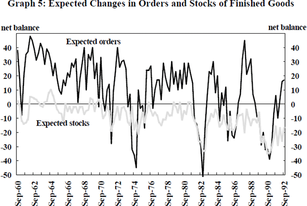
Table 6 presents the correlation coefficients between expected changes in demand and inventories of finished goods and raw materials. Each of the correlation coefficients in the table is positive and relatively large. In every case it is possible to reject the null hypothesis that the correlation coefficient equals zero. Higher expected demand leads firms to expect both higher stocks of raw materials and higher stocks of finished goods.
| Sample Period | |||
|---|---|---|---|
| 1960:3–92:3 | 1960:3–76:3 | 1976:4–92:1 | |
| Inventories of Final Goods | 0.71** | 0.58** | 0.72** |
| Inventories of Raw Materials | 0.82** | 0.78** | 0.80** |
| Note. 1. ** indicates that the correlation coefficient is statistically different from zero at the 1 percent level. |
|||
We turn now to an examination of cost shocks. Ideally, we require some measure of shocks to real production costs per unit of output. While there is no direct measure of these shocks, the survey does allow the construction of a proxy. This proxy is constructed from two questions. The first question asks firms whether they expect an increase or decrease in their average costs per unit of output. These costs are in nominal terms. In an attempt to control for increases in the price level we use a second question which asks whether the firm expects their average selling price to increase or decrease. We use the difference between the net balance response to the cost question and the net balance response to the price question as a measure of expected changes in real costs. A similar calculation is performed using the data on actual experience. Subtracting the expected experience from the actual experience provides us with our proxy for cost shocks.[16]
In Table 7 we report the correlations between these cost shocks and the shocks to inventories of both final goods and raw materials.[17] We also report the correlations between our proxy for expected changes in real costs and expected changes in stocks.
| Sample Period | |||
|---|---|---|---|
| 66:3–92:3 | 66:3–76:3 | 76:4–92:3 | |
| Correlation Between Unexpected Inventories and Unexpected Costs | |||
| Inventories of Finished Goods | 0.12 | 0.10 | 0.27* |
| Inventories of Raw Materials | −0.15 | −0.19 | −0.07 |
| Correlation Between Expected Inventories and Expected Costs | |||
| Inventories of Finished Goods | −0.32** | −0.34 | −0.58** |
| Inventories of Raw Materials | −0.29** | −0.16 | −0.58** |
| Note. 1. *(**) indicates that the correlation coefficient is statistically different from zero at the 5 (1) per cent level. |
|||
For the sample period as a whole, the correlations between the cost shocks and the inventory shocks are small and insignificantly different from zero. In contrast, over the second half of the sample period the correlation between cost shocks and shocks to inventories of finished goods is positive and statistically significant. However, this correlation is opposite in sign to that predicted by cost-shock based inventory models; it suggests that when costs are unexpectedly high, inventories are also unexpectedly high.
In contrast, the negative correlations in the second half of the table provide at least some support for the cost-shock theories. This is particularly the case over the second half of the sample period. When costs are expected to increase, firms expect both stocks of finished goods and raw materials to fall.
In estimating and presenting the above correlations it has been implicitly assumed that cost shocks and demand shocks are uncorrelated. This assumption may not be valid. When demand is weak, the costs of production may fall and when demand is strong production costs may rise. If demand and cost factors are related, the above correlations may not reflect underlying independent influences. In an attempt to isolate the independent effects of demand and supply side factors we estimate two equations. The first equation explains shocks to inventories in terms of the demand and cost shocks. The second explains expected changes in inventories in terms of expected changes in demand and expected changes in costs.
In the discussion of Graph 5 it was suggested that there may be some asymmetry in the response of inventories to expected increases and decreases in demand. Rather than imposing the constraint that the inventory response is symmetric, we allow the response to vary depending upon whether expected inventory accumulation is greater, or less than, the mean expected inventory accumulation.[18] Separate estimates for the two cases are obtained by defining two dummy variables. The first dummy (D1) takes a value of one if expected inventory accumulation is greater than the mean expected accumulation. The second dummy (D2) takes a value of one if it is less than the mean. The expected demand series is then multiplied by these two dummy variables to create two ‘expected demand’ regressors.
A similar procedure is followed for the inventory shock equation. In this case, the first dummy variable takes on a value of one if the shock to demand is greater than the mean shock. The second dummy takes on a value of one if it is less than the mean shock. The estimation results for the equations explaining shocks to inventories are presented in Table 8, while the results for the equation explaining expected changes in inventories are presented in Table 9.
| Stock of Finished Goods | Stock of Raw Materials | |||||
|---|---|---|---|---|---|---|
| 66:3:92:3 | 66:3–76:3 | 76:4–92:3 | 66:3–92:3 | 66:3–76:3 | 76:4–92:3 | |
| Constant | 8.86 (5.81) |
11.14 (2.91) |
6.68 (4.16) |
10.69 (4.93) |
13.07 (2.43) |
9.00 (3.81) |
| Demand Shock*D1 (favourable) |
−0.64 (2.30) |
−1.00 (7.45) |
0.22 (1.79) |
−0.14 (0.76) |
−0.40 (2.30) |
0.43 (2.61) |
| Demand Shock*D2 (unfavourable) | −0.10 (1.03) |
−0.15 (1.03) |
−0.11 (1.03) |
0.10 (1.02) |
0.08 (0.69) |
0.08 (0.57) |
| Cost Shock | −0.02 (0.13) |
−0.39 (1.46) |
0.24 (2.22) |
−0.16 (1.12) |
−0.43 (1.16) |
0.01 (0.10) |
 |
0.19 | 0.47 | 0.05 | 0.01 | 0.06 | 0.03 |
| H0:β1 = β2 (p-value) | 0.06 | 0.00 | 0.08 | 0.27 | 0.03 | 0.19 |

| Stock of Finished Goods | Stock of Raw Materials | |||||
|---|---|---|---|---|---|---|
| 66:3–92:3 | 66:3–76:3 | 76:4–92:3 | 66:3–92:3 | 66:3–76:3 | 76:4–92:3 | |
| Constant | −9.37 (5.64) |
−4.60 (1.49) |
−6.88 (3.60) |
−13.74 (8.40) |
−13.68 (2.45) |
−10.56 (6.28) |
| Expected Demand*D1 (favourable) | 0.18 (2.48) |
0.20 (3.07) |
0.03 (0.29) |
0.33 (4.40) |
0.36 (4.28) |
0.19 (1.67) |
| Expected Demand*D2 (unfavourable) | 0.37 (2.86) |
0.09 (1.12) |
0.47 (5.47) |
0.49 (4.40) |
0.31 (3.14) |
0.53 (5.93) |
| Expected Change in Costs | −0.11 (0.92) |
−0.26 (2.05) |
−0.28 (3.30) |
−0.02 (0.13) |
0.07 (0.28) |
−0.26 (2.07) |
 |
0.47 | 0.33 | 0.62 | 0.63 | 0.57 | 0.68 |
| H0:β1 = β2 (p-value) | 0.30 | 0.40 | 0.01 | 0.33 | 0.75 | 0.04 |
| Note. 1. T-statistics appear in parentheses below coefficient estimates. Standard errors have been calculated using the Newey-West procedure with three lags. |
||||||

Using the full sample period, the results confirm that demand shocks have had a statistically
significant effect on inventories of finished goods. The effect is significantly
stronger when demand is unexpectedly high than when it is unexpectedly low.
The coefficient on the cost shock variable is extremely small and is insignificantly
different from zero. Comparing the results for the two sub-samples, we find
significant differences in the estimates and in the ability of the equation
to explain shocks to inventories of finished goods. Over the first half of
the period the
is 0.47; this falls to 0.05 over the
second half. Over the second half of the sample period the coefficients on
both demand shock variables are insignificantly different from zero. This suggests
that unexpected changes in demand have come to play a significantly
smaller role in the inventory cycle.
The equation explaining unexpected changes in the stocks of raw materials has very low explanatory power. Over the full sample period, the demand shock variables and the cost shock variable are insignificantly different from zero. In contrast, when the sample is split in two, the favourable demand shock is significant in both sub-samples. The sign is, however, not consistent across the two periods.
The equations explaining expected changes in stocks perform considerably better. Over the full sample period, both the expected demand variables have positive and statistically significant coefficients in both the stocks of raw materials and stocks of finished goods equations. That is, when firms expect demand to increase they also expect their stocks of raw materials and finished goods to increase. Again, in both equations the cost shock variable is insignificant when using the full sample period.
For finished goods the two sample periods again show different results. Over the first half of the sample, the coefficients on favourable and unfavourable changes in demand are not significantly different from one another. In contrast, over the second half of the sample, the coefficient on unfavourable changes in demand is significantly greater than on favourable changes. Over this second half of the sample, expected declines in demand have caused large expected declines in inventories while expected increases in demand have caused negligible increases in inventories of finished goods. In addition, over the second half of the sample, expected changes in costs have a significant effect on expected inventories of the sign predicted by the cost shock models.
The results in Tables 8 and 9 suggest that changes in stocks of finished goods have
increasingly become driven by expected rather than unexpected changes in demand. The ability
of demand shocks to explain unexpected changes in inventories is much lower
over the second half of the period. In contrast, the ability of expected
changes in demand to explain
expected changes in inventories is considerably higher over the second
half of the sample. For finished goods the
increases from 0.33 to 0.62 while for
raw materials it increases from 0.57 to 0.68.
The above conclusions are robust with respect to the point at which the sample period is split. In Appendix 2 we present the estimation results for the case in which the sample period is split at the June quarter of 1982. This quarter marks the beginning of the period of a declining stocks to sales ratio (see Graph 2). The results are qualitatively the same as those in Tables 8 and 9.
Graph 5 suggests that over recent years there has been an increase in the number of firms reporting an expected decline in stocks of finished goods. This is consistent with the decline in the overall stocks to sales ratio. To remove possible distortions caused by trend movements in the expected inventory series, a linear time trend was included in the estimated regressions. The results are reported in Tables A3 and A4 in Appendix 2. The sample period is split at the June quarter of 1992. Again, the results are qualitatively similar to those presented in Tables 8 and 9. As expected the time trend variable in insignificantly different from zero in each of the ‘inventory shock’ equations. In contrast, it is negative and significantly different from zero in each of the ‘expected inventory’ equations. For both finished goods and raw materials, the absolute size of the coefficient on the time trend is larger in the second sample period. This again supports the proposition that the process of reducing stock levels accelerated over the 1980s.
The conclusion that expected changes in demand now play a more important role is also supported by a comparison of the variance of the expected changes in finished goods with the variance of the forecast error. Over the first half of the sample, the ratio of the variance of the forecast error to the variance of the expected change in inventories is 2.6; this compares with a ratio of 0.7 over the second half of the sample period.[19] In addition, not only has the relative variance of the forecast error declined but so has the absolute variance, while the absolute variance of the expected changes in inventories has increased.
Footnotes
The t-statistic for the test of the hypothesis that the average shock equals zero is 6.7. [11]
The t-statistic for the test of the hypothesis that the average shock to finished good inventories is zero is 9.3. The average shock to inventories of raw materials is 7.3 with a t-statistic of 9.2. [12]
Given this similarity, we report results using only the ‘net balance’ figures in subsequent tables. [13]
Blinder (1986) also discusses the implications of the econometrician not using the full information set. [14]
The range in the net balance figure for expected changes in stocks of raw materials is −44 to 11. [15]
This proxy for real cost shocks is less than perfect. For example, if a firm experiences no change in its cost of production but is able to increase its output price (with no change in the general price level) our measure would record a reduction in real costs. However, this would be incorrect as our measure would simply be picking up an increase in margins for the individual firm. This problem is less severe when we aggregate over a large number of firms as not all firms can increase their prices relative to the general price level. [16]
The questions concerning costs and prices were introduced in June 1966. Consequently, the sample period used to calculate correlations between inventories and costs runs from June 1966 to September 1992. [17]
This mean is calculated using data for the full sample period. Similar results are obtained if separate means are calculated for each sub-period. [18]
If 1982:2 is used as the break point these ratios are 2.2 and 0.9 respectively. [19]