RDP 9007: Operating Objectives for Monetary Policy 3. Short-run Stabilisation Properties of Alternative Rules
November 1990
- Download the Paper 841KB
This section considers three simple rules for interest rate policy which satisfy the requirements for long-run determinacy of the price level. The rules are defined as follows:
- Fixed exchange rate: et = 0
-
Price target: Rt =

- Nominal income target: Rt = γ(pt + yt).
The specifications differ from earlier treatments of price and nominal income targeting by assuming an interest rate, rather than a monetary quantity, is the policy instrument.
The aim is to compare the amount of stabilisation provided by each rule in the face of various exogenous shocks.
A convenient way to simplify the notation, for the purpose of studying the short-run properties of the model, is to assume that all shocks are temporary.[9] The model can then be written in terms of deviations from the non-stochastic equilibrium, as follows:
This short-run version of the model incorporates the usual small country assumptions: world prices are exogenous, and therefore export volumes are determined entirely on the supply side; changes to the terms of trade have explicit real income effects as well as export volumes are determined entirely on the supply side; changes to the terms of trade have explicit real income effects as well as inducing reallocation of resources between the traded and non-traded goods sectors; and changes to monetary policy, operating through the short-term interest rate, affect aggregate supply and demand in the short term, and also affect the real exchange rate. The rational expectations assumption underlying the model might be regarded as unduly restrictive, but in fact it serves as no more than a convenient stylisation which divides the analysis between the short run (the current period) and the long run (all future periods). For this purpose, the short run is to be thought of as the period within which expectations do not adjust or, alternatively, monetary policy is non-neutral; this is not necessarily very restrictive since there is nothing in the formal analysis which requires us to specify how long a “period” is.
In principle, the comparative analysis of policy rules can proceed along the following lines. First, an objective function must be defined. We assume that the objective is to minimise some weighted combination of price and output variances:
Second, for each policy rule, the model is solved and expressions for the price and output variances can be derived as functions of the variances of the exogenous shocks. These expressions are of the form:
These derivations are somewhat cumbersome, and are reported in the Appendix. Third, the welfare costs associated with price and output variances under the different policy rules can be evaluated using the objective function. In general, the ranking of policy rules on this criterion will depend on a number of factors which can only be determined empirically: for example, the configuration of model parameters, the relative sizes of the exogenous variances, and the relative weights given to price and output stabilisation in the objective function. However, it is possible, for any given shock, to rank the stabilising properties of the three rules. What follows is an informal presentation along these lines, based on the results derived in the Appendix. The exogenous shocks included in the model are considered in turn.
(a) Domestic demand shocks
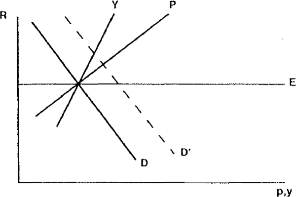
The effects of a positive shock to domestic demand are illustrated in Diagram 2. The downward sloping D curve is really a reduced form combining all the behavioural equations in the model excluding the policy rule; this implies that as the interest rate is lowered, both prices and output rise in the short term. Equilibrium for the system as a whole occurs where this curve intersects with whichever policy rule is operating. The rules are labelled E (fixed exchange rate) P (price target) and Y (nominal income target) respectively.

Starting with the fixed exchange rate case, the shock increases both prices and output in the non-traded goods sector, while output in the export sector is unaffected because there is no change in the domestic currency price of exports. The interest rate is unchanged because it is tied to the world interest rate when the exchange rate is fixed. A price targeting rule, by comparison, responds to this disturbance by raising the interest rate, thus tending to raise the exchange rate and dampen the price and output effects relative to results under a fixed exchange rate. Output is reduced in both the non-tradeables and export sectors. For a given policy parameter γ, a nominal income targeting rule raises the interest rate still further, and therefore achieves greater stabilisation of both prices and output than in either of the other two cases.
(b) Shocks to the terms of trade[10]
An upward shock to the price of exports has effects which are similar to those of a simultaneous shock to supply and demand in a closed economy. Aggregate supply is increased, and the income effect arising from the export sector pushes the demand curve for non-tradeable goods outwards, putting upward pressure on domestic prices. Both prices and output rise and, starting from the case where the nominal exchange rate is fixed, there is a rise in the real exchange rate. At an intuitive level it is fairly clear that a policy which raises the nominal exchange rate in response to this shock will dampen these price and output effects. Both the nominal income and price-targeting rules have this property.
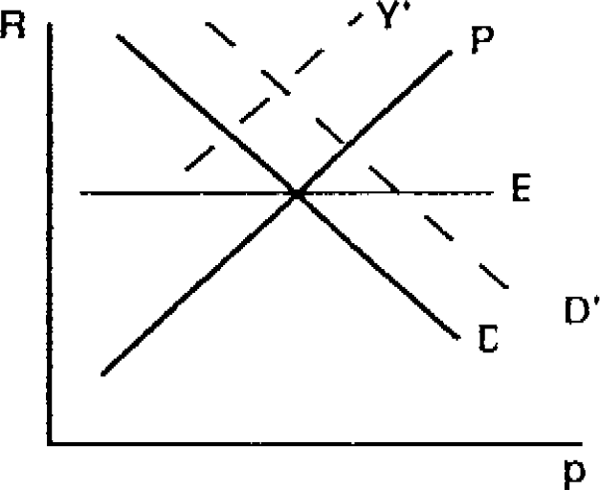
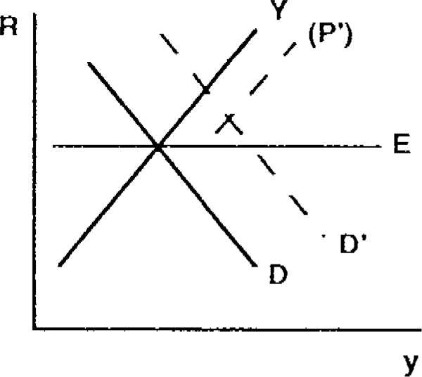
The full-system effects of the shock under the three regimes are shown in more detail in Diagrams 3 and 4. The downward sloping line in each case represents the reduced form relationship between the interest rate and either prices or output. Full system equilibrium occurs where this condition intersects with the policy reaction function; in the fixed exchange rate case, the reaction function is horizontal because policy does not respond to changes in prices or output, while in the other cases, the reaction functions are upward sloping.


In Diagram 3, the export price shock shifts outward the equilibrium R-p locus, because the increased demand for non-tradeables raises the price level for a given interest rate. Under a price targeting rule, the interest rate and exchange rate rise to offset some of this effect so that the short-run variance of the price level is reduced. A further effect of the shock is that if a nominal income target is operating, the policy reaction function is itself shifted to the left as income rises. This further raises the interest rate and exchange rate, and may actually result in the price level falling. It is shown in the Appendix that this still results in a smaller absolute change in prices than under the fixed exchange rate case, but that the relativity between variances of prices under nominal income and price targeting rules is ambiguous.
Diagram 4 shows the same disturbance in R-y space, in order to demonstrate the relative variabilities of output. In this case the ranking of policy rules is unambiguous, with the nominal income target producing the lowest output variation, and fixed exchange rates the highest.
(c) Supply shocks to the non-traded goods sector
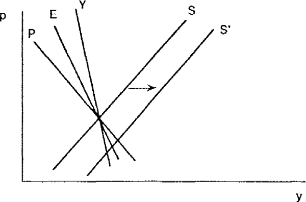
An example of such a shock would be an exogenous change in real wages, assuming the non-traded sector is relatively labour intensive. An expansionary domestic supply shock raises output and reduces prices relative to the non-stochastic equilibrium. The general equilibrium effects of such a shock can be illustrated as in Diagram 5. The curve labelled S is the supply function for non-traded goods (equation (1)), and the “demand curve” is a reduced form of the remaining equations in the model, whose slope depends on which of the three policy rules is adopted.

Taking the fixed exchange rate case as a benchmark, the reduced form demand curve is downward sloping because, other things equal, a higher domestic price level reduces real income and raises the expected real interest rate, thus lowering the demand for non-traded goods. Relative to the fixed exchange rate case, the demand curve under a price level target has a flatter slope, and hence stabilises prices more, and output less, in response to a domestic supply shock. The reason for this is that by reducing prices, an expansionary supply shock acts as a signal for interest rates to be lowered, which dampens the fall in prices but adds to the output effect. In the case of a nominal income target this result is reversed, because the net effect of an expansionary supply shock is to expand nominal income and hence to act as a signal for interest rates to be raised; this stabilises output relative to the fixed exchange rate case, but amplifies the effect on prices.
It follows from these considerations that the preferred response to a supply shock depends on the relative weights of price and output variances in the policymaker's objective function. If the objective is primarily to stabilise output, the order of preference among the three policy rules is: nominal income target, fixed exchange rate and price level target. If the short-run objective is to stabilise prices, this ranking is reversed.
(d) Summary
The conclusions from the preceding analysis are summarised, below in Table 1.
| Source of disturbance | Criterion | Ranking | ||
|---|---|---|---|---|
| 1 | 2 | 3 | ||
| Domestic demand | Output | Y | P | E |
| Prices | Y | P | E | |
| Terms of trade | Output | Y | P | E |
| Prices | E | |||
| Domestic supply | Output | Y | E | P |
| Prices | P | E | Y | |
| Export supply | Output | Y | P | E |
| Prices | E | |||
|
Notes: For each type of disturbance, the table provides rankings for the variances of output and prices under the three policy rules: a fixed exchange rate (E), price target (P) and nominal income target (Y). A ranking of 1 indicates the lowest variance. Blanks appear where the rankings are ambiguous. |
||||
Although an unambiguous preference for any one of the policy rules cannot be established from these results, a number of clear principles nonetheless emerge.
- Nominal income targeting always produces the lowest output variance among the three policy rules studied. It follows that if the weight given to output stabilisation in the policymaker's objective function is sufficiently high (f close to one), then nominal income targeting is the preferred policy rule. This preference is independent of information about the relative variances of the exogenous shocks.
- For all shocks except one (to domestic supply), the fixed exchange rate is dominated by the other two policy rules. Therefore, fixing the exchange rate can never be optimal in this analysis unless the variance of domestic supply shocks is large enough to outweigh the combined effect of terms-of-trade and domestic-demand shocks. Even then, fixing the exchange rate is inferior to the nominal income rule when f is close to one, and is inferior to price targeting when f is close to zero.
- When shocks to domestic demand are predominant, the nominal income target is unambiguously preferred over the two alternatives, giving the lowest variances for both prices and output.
Footnotes
This method was proposed by Aizenman and Frenkel (1986). [9]
The case of a supply shock to the export sector (for example, a natural resource discovery) is not discussed separately. It is shown in the Appendix that the qualitative results are identical to those for a terms-of-trade shock. [10]


