RDP 9007: Operating Objectives for Monetary Policy Appendix
November 1990
- Download the Paper 841KB
DERIVATION OF RESULTS IN SECTION 3
The full model consists of equations (I) to (VI), combined with one of the following policy rules:
| (i) Fixed exchange rate: | e = 0, which implies R = 0. |
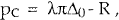
| (ii) Consumer price target: | R = γpc. |
| (iii) Nominal income target: | R = γ(p+y). |
For each choice of policy rule, the model has solutions for prices and output which are of the form


Assuming the stochastic terms are all independent, comparative results for price and output variables under the three rules can be obtained by comparing the absolute values of corresponding coefficients in the above solution equations. For example, π1 measures the effect of domestic supply shocks on the variance of output, and we aim to rank the values of π1 obtained using each of the policy rules. The procedure is then repeated for the remaining coefficients in equaztions (A1) and (A2).
To solve the model, we begin by collapsing equations (I) to (VI) down to the following two-equation system:[12]

| where π | = −(1−λ)u + (1−λ)v + w + (1−λ) (1+β)x |
 |
= (1−λ) (1+β) + αλ. |
The interest rate rules can then be expressed in terms of the exogenous shocks as follows:
- R = 0.
-
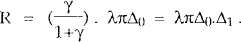
-
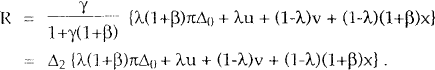 .
.
This provides sufficient information to determine the coefficients in equations (A1) and (A2). It will be useful to note that Δ1 and Δ2 are both less than one, and that Δ1 < (1+β)Δ2 < 1.
Domestic supply shock
-
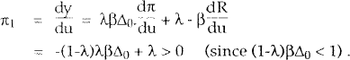
-
π2 = −(1−λ)λβΔ0 + λ + βλ(1−λ)Δ0Δ1
= −λβΔ0(1−λ)(1−Δ1) + λ, which is positive and greater than π1.
λ2 = −(1−λ)λΔ0 + λ(1−λ)Δ1Δ0
= −λ(1−λ)Δ0(1−Δ1), which is negative and less than λ1 in absolute value.
-
π3 = −(1−λ)λβΔ0 + λ + βλ(1+β)(1−λ)Δ0Δ2 − βλΔ2
= −(1−λ)λβΔ0(1 − (1+β)Δ2) + λ(1−βΔ2).
This expression is positive because 1−(1+β)Δ2 < 1−βΔ2 , and is less than π1, since (1+β)(1−λ)Δ0 < 1.
λ3 = −λ(1−λ)Δ0 + λ(1+β)(1−λ)Δ2Δ0 − λΔ2.
Here the sum of the second and third terms is negative, so λ3 is greater than λ1 in absolute value.
Export supply shock
-
π1 = λβ(1−λ)Δ0 + (1−λ) > 0
λ1 = λ(1−λ)Δ0 > 0.
-
π2 = λβ(1−λ)Δ0 + (1−λ) − βλΔ1Δ0(1−λ)
= λβ(1−λ)Δ0 (1−Δ1) + (1−λ) < π1.
λ2 = λ(1−λ)Δ0 − λ(1−λ)Δ1Δ0
= λ(1−λ)Δ0(1−Δ1) < λ1.
-
π3 = λβ(1−λ)Δ0 + (1−λ) − βλ(1+β)(1−λ)Δ2Δ0 − β(1−λ)Δ2
= λβ(1−λ)Δ0(1−(1+β)Δ2) + (1−λ)(1−βΔ2) , which is positive and less than π2.
λ3 = λ(1−λ)Δ0 − λ(1−λ)(1+β)Δ2Δ0 − (1−λ)Δ2.
This expression is ambiguous in sign, and it is also ambiguous whether or not it is smaller in absolute value than λ1 or λ2. It should be noted, however, that there exist values of the policy parameter γ for which λ3 < λ1 in absolute value: γ (and hence Δ2) can always be chosen to be sufficiently small that the second and third terms in the above expression do not over-compensate for the absolute size of the first.
Domestic demand shock
-
π1 = λβΔ0 > 0
λ1 = λΔ0 > 0.
-
π2 = λβΔ0 − λβΔ0Δ1 < π1
λ2 = λΔ0 − λΔ0Δ1 < λ1.
-
π3 = λβΔ0 − λβΔ0(1+β)Δ2 < π2 (since (1+β)Δ2 > Δ1)
λ3 = λΔ0 − λ(1+β)Δ0Δ2 < λ2 (since (1+β)Δ2 > Δ1).
Terms of trade shock
-
π1 = λβΔ0(1−λ)(1+β) + β(1−λ) > 0
λ1 = λΔ0(1−λ)(1+β) > 0.
-
π2 = λβΔ0(1−λ)(1+β) + β(1−λ) − βλΔ0(1−λ)(1+β)Δ1 < π1
λ2 = λΔ0(1−λ)(1+β) − λΔ0(1−λ)(1+β)Δ1 < λ1.
-
π3 = λβΔ0(1−λ)(1+β) + β(1−λ) − βΔ0λ(1−λ)(1+β)Δ2 − β(1−λ)(1+β)Δ2 < π2 (since (1+β)Δ2 < 1).
λ3 = λΔ0(1−λ)(1+β) − λ(1+β)(1−λ)(1+β)Δ0Δ2 − Δ2(1−λ)(1+β).
This expression has the same ambiguity of relative size as was remarked upon in the case of the export supply shock above.
Footnote
For simplicity of exposition, it is assumed that the demand elasticities g and h are equal to one, but this does not materially affect the qualitative results. [12]