RDP 8907: Tax Policy and Housing Investment in Australia 4. Simulation Results
November 1989
- Download the Paper 887KB
In this section we examine the response of home prices, land prices, rents, and investment expenditure to change in tax regimes and exogenous shocks. In particular we consider 6 simulations:
- Removal of the capital gains tax on housing;
- Cut in company tax rate by 10 percent;
- Replacing nominal interest deductibility by real interest deductibility;
- Permanent 300 basis point rise in real interest rates;
- Permanent 5 percent rise in inflation; and a
- Permanent 5 percent rise in inflation with only real interest deductibility.
These simulations all assume the policies and shocks are permanent and unanticipated. Because of the nature of this model, we can also consider the effects of policy announcements as well as temporary policy changes.
For each shock we present results for all endogenous variables for the original steady state and the new steady state. These are shown in Table 3. Note that the first column of results is the original steady state. Every subsequent column is the new steady state following the shock. Each shock is independent and so comparison should always be made with column 1. We also plot the time paths of housing investment, the price of land, the price of homes and rent.
| Base State | Capital Gains Cut | Company Tax Cut | Real Interest Deductibility | |
|---|---|---|---|---|
| pHS | 0.10 | 0.09 | 0.11 | 0.14 |
| K | 6,000,000 | 6,907,235 | 54,448,886 | 4,313,142 |
| J | 180,000 | 207,217 | 163,346 | 29,394 |
| L | 5,580,000 | 5,580,000 | 5,580,000 | 5,580,000 |
| F | 11,027,667 | 11,832,055 | 10,505,157 | 9,349,856 |
| FK | 0.92 | 0.86 | 0.96 | 1.08 |
| FL | 0.99 | 1.06 | 0.94 | 0.84 |
| I | 201,600 | 232,083 | 182,948 | 144,921 |
| q* | 1.24 | 1.24 | 1.24 | 1.24 |
| PL | 1.00 | 1.15 | 0.91 | 0.72 |
| pHome | 1.01 | 1.09 | 0.96 | 0.86 |
| i | 0.08 | 0.08 | 0.09 | 0.10 |
| mK | 1.53 | 0.93 | 1.52 | 1.51 |
| mL | 1.65 | 1.15 | 1.48 | 1.17 |
| r | 0.07 | 0.07 | 0.07 | 0.07 |
| π | 0.06 | 0.06 | 0.06 | 0.06 |
| pH | 1.00 | 1.00 | 1.00 | 1.00 |
| YN | 44,110,671 | 44,110,671 | 44,110,671 | 44,110,671 |
| Base State | Interest Rate Rise | Inflation Shock | ||
| PHS | 0.10 | 0.13 | 0.06 | |
| K | 6,000,000 | 4,614,982 | 10,211,737 | |
| J | 180,000 | 138,449 | 306,352 | |
| L | 5,580,000 | 5,580,000 | 5,580,000 | |
| F | 11,027,667 | 9,671,483 | 14,386,590 | |
| FK | 0.92 | 1.05 | 0.70 | |
| FL | 0.99 | 0.87 | 1.29 | |
| i | 201,600 | 155,063 | 343,114 | |
| q* | 1.24 | 1.24 | 1.24 | |
| PL | 1.00 | 0.77 | 1.70 | |
| pHome | 1.01 | 0.89 | 1.32 | |
| i | 0.08 | 0.10 | 0.11 | |
| mK | 1.53 | 1.51 | 1.55 | |
| mL | 1.65 | 1.25 | 2.84 | |
| r | 0.07 | 0.10 | 0.07 | |
| π | 0.06 | 0.06 | 0.11 | |
| PH | 1.00 | 1.00 | 1.00 | |
| YN | 44,110,671 | 44,110,671 | 44,110,671 |
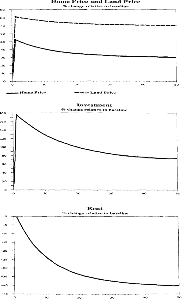
The dynamic adjustment between steady states is shown in Figures 2–6. It is seen in these figures that on the announcement of the policy there is an initial rise and overshooting of the land price because of the increased attractiveness of housing relative to other assets. Overshooting occurs because the stock of housing can only adjust slowly whereas prices can jump. The initial rise of 18 percent is followed by a gradual convergence to just under 15 percent higher in the new steady-state. The home price also overshoots, rising by over 12 percent initially and then falling back towards 8 percent higher as the supply of homes increases forcing down rents. The surge in housing activity is illustrated in the investment results. The rent graph shows a gradual fall in rent corresponding to a gradually rising supply of homes.
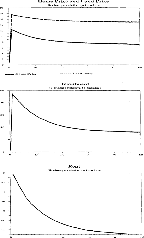
a. Removal of Capital Gains Tax on Housing
In this simulation we assume the capital gains tax is reduced from 30 percent to zero in period 1. The consequences of this for the steady state is shown in column 2 of Table 3. The new steady state has a larger stock of houses which implies a larger stock of homes, higher home prices and land prices and lower rent.
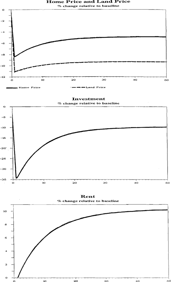
b. Cut in company tax rate by 10 percent
In the second simulation we assume that the marginal tax rate on the income of housing investors falls from 40 percent to 30 percent. The new steady state resulting from this shock is shown in column 3 of Table 1. Recall that inflation is set at six per cent per annum. Lowering tax decreases the size of the inflation tax distortion and therefore decreases the housing subsidy. In this case we get the opposite to the removal of the capital gains tax. Land prices, home prices and investment fall initially but then rise over time to a new steady state with lower prices, higher rent and a smaller housing stock. When the marginal tax rate falls housing as a form of investment becomes relatively less attractive because the taxation advantages of housing become less important.
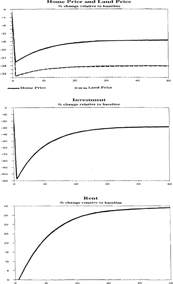
c. Replacing nominal interest deductibility by real interest deductibility
Inflation is important in this model because nominal interest payments are deductible for housing investors. In this section we simulate the removal of this policy and its replacment by real interest deductability. We see from column 4 of Table 3 that the effect of this policy on the new steady state is to reduce the housing stock and with it the price of homes and land. Rent on the other hand rises in the new steady state reflecting the fall in rental accomodation.
In Figure 4 we again see an overshooting of prices in response to the shock. Home prices intially fall by over 25 percent before rising back to 16 percent below the previous level. Investment is also severely hit by the policy. Rent rises gradually over time as the existing stock of homes falls. Note that the effect of this policy is more pronounced than simply lowering tax rates.
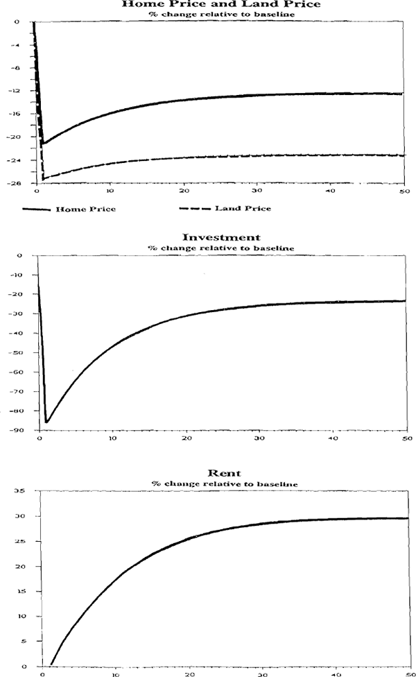
d. Permanent 300 basis point rise in real interest rates
In this simulation we assume that real interest rates rise permanently by 300 basis points. The result is quite intuitive. The new steady state shown in column 6 of Table 3 has a lower stock of homes as investors substitute away from housing into other assets. In Figure 5 we show the dynamics of adjustment. Note that home prices initially fall by 20 percent before gradually rising to around 13 percent below their intial level.
e. Permanent 5 percent rise in inflation
The results for a rise in inflation are given in column 7 of Table 3 and Figure 6. The steady-state consequences of the shock are noticably different to the real interest rate shock. In the case of the inflation shock, the distortion caused by the tax system leads to increased demand for investment housing which drives up the price of land and homes and drives rent down as the new stock of homes is constructed.
The interesting comparison between this shock and the real interest rate shock is that both lead to a rise in nominal interest rates. So we have a result where a rise in nominal interest rates leads to a fall in investment and a case where the same rise could lead to a rise in housing investment. The important distinction is whether the change in nominal interest rates reflects expected inflation, or a rise in real rates.
f. Permanent 5 percent rise in inflation with only real interest deductibility
The results for an inflation shock without nominal deductability are not shown because nothing happens to any real variables. All nominal variables change by the rate of inflation.