RDP 8608: Exchange Rate Regimes and the Volatility, of Financial Prices: The Australian Case 2. The VAR Methodology

In general we will be concerned with an (nxl) vector of n endogenous variables Y_t containing domestic and foreign financial price variables. We assume that Y_t is generated by the m^th order vector-autoregression,

where D_t is a (nxl) vector representing the deterministic component of Y_t (generally a polynomial in time), B_t are (nxn) matrices and ε_t is a (nxl) vector of multivariate white noise residuals (or innovations). Equation (1) is specified and estimated as an “unrestricted reduced form”. As is the hallmark of VARs, there are no exclusion restrictions within the B_j matrices. Rather, the B_j's are uniquely determined under the orthogonality conditions E(ε_t) = 0 and E(Y_t−jε_t) = 0, j=1, …, m, and are estimated by ordinary least squares. Given the choice of variables in Y_t, the only pretesting involved with the fitting of equation (1) is in choosing the appropriate lag length m. In general we choose the smallest m such that ε_t is indistinguishable from a multivariate white noise process.^[7]

Tests which are commonly applied to VARs are tests for Granger-causality which test whether a variable, say Y_1t is useful in forecasting another variable, say Y_2t. The variable Y_1t, is said to be useful in forecasting Y_2t if the inclusion of lags of Y_1t in the equation for Y_2t significantly reduces the forecast variance. Thus it tests whether lags of Y_1t contain any additional information on Y_2t which is not already contained in the lags of Y_2t itself.

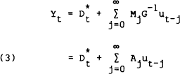
The model presented in equation (1) is difficult to describe in terms of the B_j coefficients. The best descriptive devices are the innovation accounting techniques suggested in Sims (1980, p.21) and described by Litterman (1979, pp.74–85). The first of these techniques of innovation accounting are the impulse response functions which describe the dynamic response of variables in the VAR to an impulse in one of the variables. To understand these impulse response functions, consider the moving average representation of equation (1), obtained by repeated back substitution for Y_t−1,

where M_j is a (nxn) matrix of moving average coefficients. The response of the i^th variable to a unit innovation in the k^th variable j periods earlier is given by the ik^th element of M_j. In general, however, there is likely to be some contemporaneous correlation among innovations, which is not taken into account in equation (2). If one can assume some contemporaneous causal ordering of the variables in Y_t (such that contemporaneous causality is one way, i.e., recursive) one can obtain orthogonalised innovations u_t, where u_t = Gε_t, so that E(u_t) = ϕ where ϕ is a diagonal (nxn) matrix. For example, if we have a VAR with a foreign variable and a domestic variable and assume that the domestic variable does not contemporaneously cause the foreign variable, then the foreign variable will be ordered above the domestic variable in Y_t and G will be of the form,

where ρ is the estimated coefficient in the regression equation,

ε_1t is the innovation in the foreign variable, ε_2t the innovation in the domestic variable and u_2t the orthogonalised innovation in the domestic variable (in the sense that it is orthogonal to u_1t = ε_1t).

In terms of orthogonalised innovations, u_t, the moving average representation is,

where the ik^th element of A_j gives the response of variable i to an orthogonalised unit impulse in variable k, j periods earlier.

For the purposes of this paper, however, the second device of innovation accounting will be used. This relates to the decomposition of the k-step ahead forecast variance of each variable in the VAR, into percentages contributed by the innovations in each variable. A variable whose own innovations account for all or most of its own forecast variance would be said to be exogenous (in the Sims sense) to the system.

The k-step ahead forecast variance may best be seen by considering the k-step ahead forecast error induced by forecasting Y_t linearly from its own past,

(in terms of orthogonalised innovations) where E_t (Y_t+k) is the linear least squares forecast of Y_t+k given all information at time t. The k-step ahead forecast variance is,

Because of the extensive orthogonality conditions built into the model, the k-step ahead forecast variance of each variable will be a weighted sum of the variances of the innovations to each variable. Thus we can obtain the percentage contribution of each variable's innovations to the variance of any other variable.

Footnote

On the basis of tests for within, and across, equation serial correlation and tests for the significance of B_m, from the zero matrix. The inverse autocorrelation function (i.e., the autocorrelation function of the dual model) is used to test for non-stationarity of the residuals. (See, for example, Priestley (1981).) All of the empirical work is done using the macro facilities of version 5 of SAS. [7]