RDP 2012-05: Payment System Design and Participant Operational Disruptions 4. Methodology
September 2012 – ISSN 1320-7229 (Print), ISSN 1448-5109 (Online)
- Download the Paper 578KB
4.1 The Simulator
The Bank of Finland has developed a versatile Payment and Settlement System Simulator (BoF-PSS2) for modelling the complex interactions that occur in payment and settlement systems. Simulations can be used for analysing the implications for liquidity and risk of changes in system functionality, market structure, and settlement rules or conventions, as well as the effect of specific events (such as a participant's operational disruption). Broadly, the Bank of Finland simulator mimics the functionality of RTGS systems; it requires the user to input transaction, liquidity and other data, which are then processed according to specified algorithms that simulate the workings of an actual RTGS system. The simulations generate a wide range of transaction-level and aggregated data, such as the time that each transaction was settled and the value of unsettled payments at the end of a day.
4.2 Data
Our simulations are based on RITS transaction, liquidity and sub-limit data from 10 business days in the first quarter of 2008. This period is representative of a typical fortnight in 2008. During this period there was an average of $191 billion settled each day using around $15 billion of liquidity (i.e. each dollar was used to make an average of 13 payments each day), compared with a daily average of $195 billion using around $17 billion in 2008 as a whole. The value of payments settled on a particular day in our sample ranges from $96 billion to $247 billion, with a sample standard deviation of $41 billion, compared with a standard deviation of $38 billion for 2008 as a whole.
4.3 System Design
To measure the marginal benefit of hybrid features during an operational disruption, participant-level disruptions are simulated under five different system designs (Table 1). Since hybrid features usually require a central queue, all system designs, other than the pure RTGS system, incorporate this feature. Like RITS, the RITS replica has a combination of a central queue, a bilateral-offset algorithm and sub-limits. To roughly disentangle the effects of sub-limits and bilateral offset, a system with only sub-limits and a system with only bilateral offset are examined. Rather than using the existing algorithms in the simulator, this paper uses modified algorithms that more closely match the bilateral-offset algorithm and sub-limit features in RITS (see Appendix A for further details).
| Central queue | Bilateral offset | Sub-limits | |
|---|---|---|---|
| Pure RTGS | – | – | – |
| Central queue only | √ | – | – |
| Bilateral offset | √ | √ | – |
| Sub-limits | √ | – | √ |
| RITS replica | √ | √ | √ |
4.3.1 Submission times
While a change in system design is likely to provide an incentive for participants to vary submission times, for simplicity this paper generally assumes that there is no change in submission behaviour.[8] However, since there is no central queue to coordinate payments in a pure RTGS system, participants require some internal mechanism to ensure that a payment is only sent to the RTGS system when the participant has sufficient funds to settle that payment. Consequently, RITS submission times are unlikely to be appropriate when simulating a pure RTGS system. Instead, settlement times from the benchmark simulations of the central-queue-only system are used to proxy the submission times in the pure RTGS system.[9] As a result, the key difference between the pure RTGS and central-queue-only simulations is the payments on the queue. This set-up is likely to underestimate the benefits of a central queue since the visibility of queued receipts on a central queue can decrease participants' uncertainty regarding their future liquidity requirements and thereby reduce their incentive to delay submitting payments.[10]
The assumptions regarding submission time are also likely to understate the benefit of a bilateral-offset algorithm and sub-limit functionality, since inclusion of each of these features provides an incentive to submit payments earlier. A bilateral-offset algorithm reduces the incentive to submit payments late by potentially lowering the amount of liquidity required to settle payments, especially in combination with sub-limits that allow participants to reserve liquidity for time-critical payments.
4.3.2 Liquidity
As noted above, participants may decrease their holdings of liquidity in response to the inclusion of liquidity-saving algorithms, thus potentially negating the benefit of such features in the event of an operational disruption. Consequently, we report results based on actual liquidity from RITS and assume that participants decrease their holdings of liquidity by 30 per cent in response to the presence of the bilateral-offset algorithm.[11] For the latter simulations, participants' actual shares of liquidity are maintained, as this should be a reasonable indicator of each participant's relative access to liquidity.
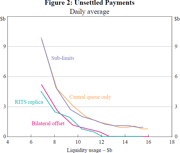
A 30 per cent reduction in liquidity was selected after analysing the effect of varying available liquidity on the value of unsettled payments in each of the four system designs with a central queue (Figure 2). As expected, the bilateral-offset algorithm significantly decreases the liquidity required to settle payments. However, an extremely large increase in liquidity would be required to settle all payments in systems that do not incorporate the bilateral-offset algorithm. Consequently, liquidity in the RITS replica and bilateral-offset systems is scaled down by 30 per cent to equalise the value of unsettled payments across all system designs at around $1.5 billion.
4.3.3 Sub-limits
In general, observed behaviour in RITS (i.e. sub-limits and payment status) is replicated when simulating systems with sub-limit functionality. However, it is reasonable to assume that participants will use all available liquidity to settle any payments outstanding at the end of the day; therefore sub-limits are reduced to zero shortly before the system closes to allow as many payments to settle as possible.
4.4 Measuring the Effect of a Disruption
The primary statistic used to measure the impact of an operational disruption is the average total value of unsettled payments each day.[12] Given that the focus is on the systemic impact of a disruption, the measure of unsettled payments excludes payments to or from the stricken participant.[13] In addition, the value of the liquidity sink, measured as the stricken participant's end-of-day balance after repaying any intraday repos, is reported.
4.5 Simulation Scenarios
In analysing the interaction between system design and participant reaction time, this paper follows the methodology used by Glaser and Haene (2009), who build on the approach established by Bedford et al (2005), to find the time when the largest ‘theoretical liquidity sink’ will form in RITS.[14] The theoretical liquidity sink is defined as follows:

where i is the stricken participant, Balanceit is participant i's balance at the central bank at time t, Receiptsit is the value of receipts it is due, Value on Queueit is the value of its outgoing payments on the queue and R represents the time it takes non-stricken participants to react. When identifying the largest theoretical liquidity sink, it is assumed that non-stricken participants take two hours to react to the operational disruption and that the disruption to participant i's payments lasts until the end of the day.
Since system design affects exactly when payments settle, the simulation starts from the point of the disruption to ensure that the results across systems are comparable. As a result, for any given day simulated, the same payments are outstanding at the start of the simulation, regardless of the system design. Benchmark simulations, in which there is no operational incident, are run for each day using each system design in order to allow unsettled payments resulting from the changes in system design to be identified; this results in five scenarios, one each for the five types of system design under consideration.
An operational disruption, at the participant and time identified using the method above, is then simulated with three different reaction times – participants reacting by stopping payments to the stricken participant after 10 minutes or 2 hours, or not reacting at all.[15] These three reaction times are modelled for each of the five system designs, with scenarios covering all relevant combinations of assumptions (Table 2). For the pure RTGS and central-queue-only systems, the only relevant assumption is the reaction time, as these systems do not include sub-limits or bilateral offset, therefore three scenarios are modelled for each of these two systems.
| System design | Reaction time | Liquidity | Sub-limits | Number of scenarios |
|---|---|---|---|---|
| Pure RTGS | 3 | na | na | 3 |
| Central queue only | 3 | na | na | 3 |
| Bilateral offset | 3 | 2 | na | 6 |
| Sub-limits | 10 minutes | na | 2 | 2 |
| 2 hours | na | 2 | 2 | |
| No reaction | na | na | 1 | |
| RITS replica | 10 minutes | 2 | 2 | 4 |
| 2 hours | 2 | 2 | 4 | |
| No reaction | 2 | na | 2 |
The liquidity assumption is relevant to systems that incorporate the bilateral-offset algorithm. Consequently, in the RTGS system with bilateral offset the three reaction times are simulated using both actual liquidity and a 30 per cent reduction in liquidity. This results in six scenarios being simulated (i.e. three reaction times × two liquidity assumptions).
In systems with sub-limits, two additional reactions to the disruption are considered. In the first case, it is assumed that participants react by not only stopping payments to the stricken participant, but also by dropping their sub-limits to zero to maximise the liquidity available to settle payments between non-stricken participants. In the second, it is assumed that participants do not drop their sub-limits. As the sub-limit assumption is irrelevant if there is no reaction, this means that five scenarios are simulated using the RTGS system with sub-limits for each day in the sample period.
For the RITS replica system, all three assumptions are relevant. For the 10-minute and 2-hour reaction times, both liquidity and sub-limit assumptions are modelled, resulting in four scenarios for each of these two reaction times. When it is assumed that participants do not react, only the two liquidity assumptions are relevant, resulting in a further two RITS replica scenarios.
In addition, this paper also investigates how system design affects the relationship between the size of the participant experiencing the operational disruption and the systemic effects of that disruption. This involves conducting a further set of simulations for the largest 15 participants (measured by value of payments submitted and received).[16] These simulations use a 2-hour reaction time, as anecdotal evidence suggests that this is the approximate time it takes participants in RITS to react to an operational disruption. As the value of queued payments varies at different times of day, disruptions at 9.15 am, 12.00 pm and 3.00 pm are modelled in these participant-size scenarios. Varying the time of day, the participant affected and the system design requires running 225 different scenarios for each day simulated (i.e. 3 times x 15 participants x 5 system designs).
Footnotes
The submission times and status of payments that experience status changes between submission and settlement in RITS have been amended to best replicate when these payments settle, as the option to change payment status is not available in the simulator. See Appendix A for further details. [8]
In addition, as simulations cannot incorporate the re-submission of payments that do not settle immediately in a pure RTGS system, the central queue model (with adjusted submission times) is used to simulate the pure RTGS system. Payments that do not settle immediately are queued and re-tested for settlement at a later stage, as if they had been re-submitted. [9]
RITS provides each participant with real-time information on their queued payments and receipts. In order to prevent participants incurring credit risk by crediting their customers before interbank settlement has occurred, the receiving participant does not receive details of the ultimate beneficiary until the payment has settled, although the paying and receiving participant are identified. [10]
In the ‘actual liquidity’ simulations, we assume that participants do not unwind intraday repos until the end of the day to minimise the effects of changes in the timing of settlement in the simulations. This is a reasonable assumption if the main driver of the cost of liquidity is the maximum value of collateral used, rather than the length of time during the day that the securities are used. For simplicity, we allow unlimited liquidity for the RBA, CLS Bank and the settlement accounts of the equity and futures clearing and settlement systems. [11]
The impact of an operational disruption could have been measured in an equivalent fashion using the value of additional liquidity required to settle all transactions. Another measure of the systemic impact is the simulator's settlement delay indicator. [12]
Note that changing the system design (without an endogenous response to this by participants) can result in unsettled payments due to insufficient liquidity, even without simulating a participant operational disruption. As a result, the value of unsettled payments, particularly in systems without bilateral offset, may be slightly overstated. [13]
In common with Bedford et al, the largest theoretical liquidity sink is restricted to the morning to ensure that there is a significant value of payments to settle after the disruption. [14]
Due to technical limitations, we are unable to prevent priority payments submitted before the time at which participants react from settling. [15]
Excluding the RBA, CLS Bank and the settlement accounts for the equity and futures markets. [16]