RDP 9310: Explaining the Recent Performance of Australia's Manufactured Exports Appendix C: Regression Results
August 1993
- Download the Paper 109KB
| Variable | Lag | Coefficient | t-statistic | H0:explanators jointly zero |
|---|---|---|---|---|
| constant | 2.9424 | 0.8 | ||
| t | −0.0009 | −0.3 | ||
| (t−64)D | 0.0111 | 3.6 | ||
| x | t−1 | 0.4117 | 4.3 | |
| x | t−2 | 0.0649 | 0.7 | |
| x | t−3 | 0.2601 | 2.7 | |
| x | t−4 | −0.0685 | −0.9 | |
| twi | t | −0.0253 | −0.2 | |
| twi | t−1 | −0.1236 | −0.6 | twi |
| twi | t−2 | −0.4487 | −1.6 | χ2 calc =16.92 |
| twi | t−3 | 0.8388 | 2.7 | p-value=0.0047 |
| twi | t−4 | −0.3994 | −2.3 | |
| protect | t | 1.6900 | 2.3 | protect |
| protect | t−1 | 1.7362 | 2.3 | χ2 calc =24.53 |
| protect | t−2 | −1.9943 | −2.8 | p-value=0.0000 |
| tp | t | 0.3461 | 0.9 | tp |
| tp | t−1 | −0.1495 | −0.3 | χ2 calc =31.81 calc |
| tp | t−2 | 0.5512 | 1.4 | p-value=0.0000 |
| gne | t | −0.2826 | −0.9 | |
| gne | t−1 | −0.1958 | −0.5 | gne |
| gne | t−2 | −0.0260 | −0.1 | χ2 calc =8.37 |
| gne | t−3 | −0.2530 | −0.5 | p-value=0.14 |
| gne | t−4 | 0.4425 | 1.3 |
GNE was excluded on the basis of these tests (with α =.05). A Bewley Transformation of the ADL was then estimated using xt−1 as an instrument for Δxt. The long-run coefficients cited in the text were then obtained. Even in the presence of a cointegrating relationship, the calculated test statistics in the Bewley transformation are not necessarily t-distributed. However, in small samples they may outperform the Phillips-Hansen fully modified estimator as Inder (1991) has shown. In any case, the model was also run in difference form. Both the insignificance of gne and the significance of the broken trend were verified.
A test for cointegration due to Kremers et al. (1992) rejects the null hypothesis of no cointegration at the 5 per cent level (test statistic, −5.3). The sum of the coefficients on t and (t − 64)D is approximately 0.01, implying that the broken trend after March 1986 adds 1 per cent per quarter (around 4 per cent per annum) onto export growth. That is, the conventional explanators explain roughly three quarters of the 16 per cent per annum average growth in manufactured exports since 1986.
An examination of the time series properties of exports indicates that the series is explosive[56]. The Phillips-Peron Zt test, with a constant and no trend, rejects the null of a unit root in favour of the alternative that the series is explosive at the 5 per cent level (test statistic, 2.7190). Four lags are sufficient to eliminate autocorrelation for the Augmented Dickey-Fuller test. The null is rejected in favour of an explosive series at the 5 per cent level (test statistic, 1.98).
The conclusion that exports are explosive is highly suggestive of a structural break. Therefore, Peron's test for stationarity around a broken trend is an appropriate diagnostic procedure. The test requires that a structural break be imposed a priori. The first quarter of 1986 is used because both the McKinsey report and the sample survey in this paper indicate that many firms commenced exporting around then. The null that the series has a unit root around a broken trend is not rejected at the 5 per cent level (test statistic, −0.1627). Given this result, it became a prior that the final model should have a significant structural break. There were versions of the model where the structural break was insignificant and the exchange rate had a very high exchange rate elasticity, but these were abandoned because the time series properties of the model became very unclear.[57]
Heteroskedasticity and autocorrelation were often problems in the various versions of the ADL. Increasing the lag lengths[58] fails to remedy autocorrelation and the resultant loss of degrees of freedom creates other problems.[59] Therefore, the preferred version of the model is estimated using a Newey-West correction for serial correlation and heteroskedasticity[60]. The presence of serial correlation in the estimated model implies inconsistent estimates because of the presence of a lagged dependent variable. Therefore the model was estimated using instrumental variables. The somewhat unorthodox instrument used for exports was the broken trend. The significance of the broken trend was established as was the insignificance of gne.
The real exchange rate is used to capture changes in PW relative to PL in the model. Conventional measures of relative prices exhibit a perverse negative correlation with the broken trend.[61] Including one of them in the regression introduces multicollinearity and implies a significant role for relative prices, but of the wrong sign. This is mistaken both from a theoretical and practical point of view. Some exporters contacted in the survey clearly stated that relative prices were instrumental in their decision to export.[62]
A modified version of the Chow predictive failure test is useful for ascertaining the extent to which a model explains groups of observations. Several dummy variables are used to entirely explain a group of observations. The joint significance of the dummies is then tested. A model which fits the data well is not improved greatly by the inclusion of the dummies. Conversely, significant dummies indicate that a model does not easily explain the observations in question.
For this particular model, successive regressions are run starting at the beginning of the data set. In each regression four consecutive observations are ‘soaked up’ by four dummies. After testing their joint significance, the same procedure is repeated with four new dummies advanced one time period. The results from these ‘rolling dummies’ regressions are summarized in the following figure.
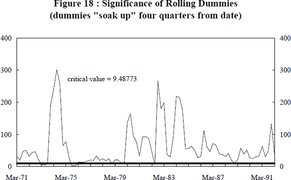
These results imply that estimating the model over sub-periods could generate different coefficient estimates. This suspicion is borne out when the above model is estimated over the sub-period December 1974 to December 1992. This period is chosen because it excludes the effects of the massive 6 percentage point reduction in the effective rate of assistance to manufacturers in December 1973. Estimating the model over this period gives the long run coefficients in the text.
Given this feature of the model, the temptation is to estimate over the period that gives the best results. Therefore a discipline imposed on the procedure is that the preferred model uses the maximum amount of data available. Otherwise the exercise takes on an entirely ad hoc character.
Given the problems of serial correlation and parameter instability, the estimated model cannot claim to be a full representation of export supply. However, the most important results are robust to different specifications. A break occurred in 1986 and gne does not, in general, explain manufactured exports.
Footnotes
That is, a time series model of x has the lagged-dependent variable coefficient significantly greater than unity. [56]
With a structural break on the RHS of the equation, premultiplication by the orthogonal projection matrix M (with X being the broken trend) collapses the problem into modelling an I(1) series. Without the structural break, an explosive series is being modelled. Inference is therefore unclear. [57]
The variables gne and twi appear in the model with four lags, indicating that adjustments to shocks takes considerable time. Somewhat arbitrarily, the variables tp and protect appear with two lags because it is judged that they are easier to adjust to. It is assumed that they can be foreseen to a greater degree. [58]
In some estimated versions increasing the lag length appeared to make autocorrelation worse, and, reduces the significance of other estimated parameters. [59]
In RATS, the command is (robusterrors,lags=8,damp=1). Eight lags are used because it is judged that this is a reasonable time for dynamic adjustments to occur. LM tests indicate that serial correlation of this order was a problem in some cases. [60]
px/pgne is a proxy for the ratio of the domestic price of manufactured exports to the domestic price of non-traded manufactures. If pman is the local price of manufactured goods, px/pman measures the incentive for a firm to export its output rather than sell it locally. Both relative prices trended down over the sample period with a pronounced downturn since the mid-1980s, coinciding with the export boom. [61]
It may be that the relative price movement reflects declining Australian productivity vis a vis the rest of the world. However, the puzzle remains as to why some survey respondents indicated that they exported because of relative price differentials. (A case in point was a capital goods firm which started to export because the local price of its output fell considerably more than the export price). In the end it was decided to use the real exchange rate because its movements accorded with the survey evidence suggesting that export profitability must have recently improved. [62]