RDP 9310: Explaining the Recent Performance of Australia's Manufactured Exports 4. Evidence of Hysteresis
August 1993
- Download the Paper 109KB
The shocks examined in the theoretical framework were chosen because they occurred in the 1980s. In this section, it is asserted that the sunk cost model adds to the understanding of the recent growth in exports. Then evidence is brought to bear on that assertion.
4.1 History in Terms of the Model
The 1982/83 recession had little effect on exports. The model suggests a possible explanation for this; exporters faced a price differential in the band of inaction. Though the recession would have tended to reduce profits from domestic sales, the exchange rate may not have been low enough to generate export profits sufficient to cover sunk costs.
The historic depreciation in the mid-1980s was a catalytic event for would-be exporters. In the sunk cost model, the world price (in local currency) rose to an extent that encouraged firms to pay their sunk costs and export for the first time.[22] Even though the exchange rate movement was partly reversed in the latter half of the decade, the model predicts that firms that had paid their sunk costs would tend to remain in their established markets. The strength of this alleged hysteretic effect depends on the exchange rate expectations of the individual firms at that time. Optimistic firms may have believed that the favourable shock would persist. These firms would have had a narrower band of inaction because the expected present value of exporting would have been unrealistically high. Note the following statement made at that time by Senator Button:
‘Manufacturers should be making their investment plans on the basis that the dollar will remain very close to its current levels and that the Government will successfully influence the course of wage and price growth to preserve gains we have made in international competitiveness’ (quoted in Dunkerly 1986, p.80).
However, other commentators, such as Dr. E. Shann, were more cautious:
‘… eventually our real exchange rate will rise. There is thus a window of opportunity for manufacturers with short lead times to earn profits. However, for projects with longer lead times there is a risk of the real exchange rate rising before they have recouped their costs, or paid off the overheads involved in establishing markets overseas’ (Shann 1986, p.15).
In the sunk cost model, the recent recession could have had a different effect on aggregate exports than the 1982/83 recession. This is because the exchange rate was lower, overall, than it was in the early 1980s. All other things held constant, PW−PL was closer to the upper bound of the band of inaction. Slack domestic demand could have put downward pressure on prices in both recessions, but expected export profits in the early 1990s may have been relatively greater by virtue of the lower exchange rate.
The model can explain some of the surge in exporting since the mid-1980s by the vanguard effect. Responding to the depreciation and the recession, pathbreaking firms established themselves in overseas markets. Their presence reduced entry costs for subsequent firms. Furthermore, the influence of the tariff reductions, begun in the early 1970s, at some point began to have an influence. The efficiency gains from using imported inputs steadily improved the competitiveness of exporters. However, in the sunk cost model, the effect on exports could have been sudden, as the threshold was reached, rather than steady.[23]
4.2 Methodology
Empirical analysis of sunk cost models is difficult. A comprehensive analysis would seem to require (unavailable) cost data for firms over a wide range of industries. There is the added difficulty of modelling export equations, which has traditionally met with little success.[24] As a result, the literature tends to focus on hysteresis in imports. Econometric validation of various models, if it exists, rests on limited evidence, such as the significance of structural breaks.[25]
The approach adopted in this paper is to have a simple model which is open to the scrutiny of testable implications. Many of the implications of the sunk cost model, including the existence of a structural break, are observed in the data. With this a case is built for the sunk cost model and hysteresis. The difficulties experienced in modelling exports motivate a sample survey. The results of the survey are consistent with the econometric results.
At the outset, a distinction is made between building a case for the sunk cost model, on the one hand, and building a case for hysteresis on the other. These beliefs are discussed separately for both the survey and the econometric evidence. First, evidence is presented in support of the sunk cost model. However, even if sunk costs can be shown to have been important, the economy may not have received the sequence of shocks necessary to change the local supply curve. That is, evidence in favour of the sunk cost model is necessary but not sufficient to establish hysteresis. The second step, therefore, involves examining export growth since the mid-1980s in light of the sunk cost model. Armed with a prior about the correct model, statistical evidence builds a case for hysteretic effects.
4.3 A Sample Survey of Manufacturing Exporters
A small scale survey was carried out to establish the importance of sunk costs. AUSTRADE provided the first 100 exporters from an alphabetical listing of its database. The listing was confined to companies in NSW with annual export revenue of between $2 million and $50 million.[26] These firms were contacted in alphabetical order until 30 successful interviews occurred.[27] This procedure approximates a random sample of Australian exporters that export between $2 million and $50 million.[28]
The survey supported the existence of a vanguard, where pathbreaking exporters reduce sunk costs for subsequent entrants. For example, some respondents argued that the profile of Australian goods established by the vanguard made subsequent entry easier. Other respondents indicated that the vanguard helped new firms by passing on information at industry forums or in networks.[29]
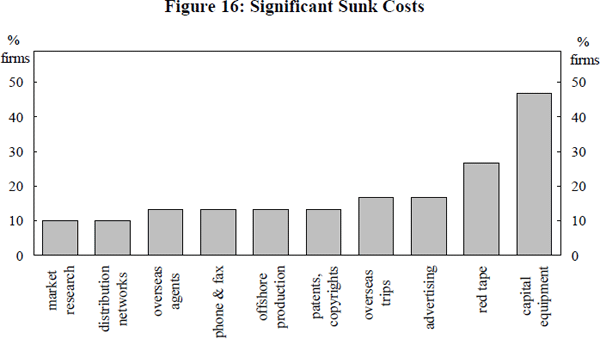
The survey respondents indicated that there were large one-off fixed costs. At the 5 per cent level, it was established that more than half the firms had at least one significant sunk cost.[30] The most significant individual sunk costs were in the area of export-related plant and equipment.[31] Even if the size of these costs are exaggerated, the analysis of Dixit (1989) has an important point to make. The combination of sunk costs and uncertainty means that large economic shocks may be necessary to change market structure. This implies that the sunk cost model is more realistic than the standard model. Armed with this prior, the late-1980s export surge is now given a sunk cost interpretation.
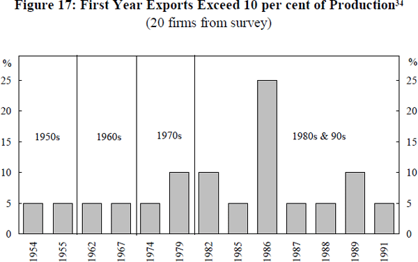
The exchange rate was nominated by 60 per cent of firms as being an important factor in their initial export decision.[32] Furthermore, the survey shows that one quarter of firms currently exporting began in 1986, the year of an historic $A depreciation.[33] If the sunk cost model is correct, this could signify that the depreciation enabled a large number of firms to cover their sunk costs and establish beachheads.
The survey also indicated that the most recent recession has had a greater impact on exports than any other recession. Of the respondents, 40 per cent indicated that they had significantly increased their exports in response to it. (Only one firm indicated that a previous recession had caused a significant increase in exports.[35])
The importance of the last recession is consistent with the description of hysteresis in the late 1980s. The combination of slack domestic demand and a (generally) lower exchange rate pushed PW−PL above d, increasing the discounted future stream of export profits to the point where paying sunk costs was optimal.
4.4 An Export Supply Equation
In an attempt to gather evidence for sunk costs and hysteresis, the following model of manufactured exports was estimated using quarterly data from March 1970 to December 1992:
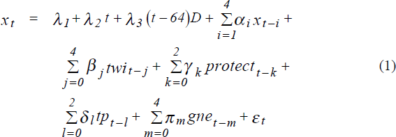
The following notation applies:
| t | – | a time trend |
| D | – | a dummy variable which takes the value unity on and after March 1986 (the 65th observation) |
| protect | – | the effective rate of assistance to manufacturers[36] |
| x | – | real manufactured exports (logarithm) |
| twi | – | the real trade-weighted exchange rate (logarithm) |
| tp | – | trading partner's industrial production index weighted by exports (logarithm). (Moving weights capture the recent switch to Asia[37]) |
| gne | – | real GNE (logarithm) |
A full list of estimates is provided in Appendix C.[38] The variable gne was found to be insignificant (p-value = 0.14). The following long-run estimates from a reparameterisation (a Bewley transformation) were obtained after gne was excluded:
| Variable | Elasticity | t-Statistic |
|---|---|---|
| twi | −0.6701 | −1.7 |
| tp | 1.6896 | 2.0 |
| protect[39] | 4.8034 | 3.8 |
As expected, exchange rate depreciations and world growth increase export volumes. The perverse sign of the coefficient measuring the effective rate of assistance results largely from an inexplicably strong decline in exports in the early 1970s, coincident with the large tariff reductions. To remove the effect of this episode, the model was re-estimated from December 1974 and the following estimated long-run coefficients were obtained:
| Variable | Elasticity | t-Statistic |
|---|---|---|
| twi | −0.2048 | −0.9 |
| tp | 0.2335 | 0.3 |
| protect | −3.6640 | −1.3 |
This table illustrates the difficulties involved in modelling exports that were alluded to earlier. Though the significance of the parameters suffers substantially from the shorter estimation period, the main point to be made is that the declines in protection explain most of the growth in exports in this regression. The surprisingly low elasticities for the exchange rate and the growth of our trading partners may be the result of the timing of the late 1980s tariff cuts, which mirrored the export surge.[40] The true values of the elasticities probably lie somewhere between the sets of estimates generated over the different sample periods. Having examined the properties of the export equation, it is now shown that it provides some evidence for the importance of sunk costs and the existence of hysteretic episodes in the late 1980s.
Econometric validation of sunk costs requires testing for a ‘hurdle’ that exporters must surmount. Krugman (1989) argues that sunk costs should make trade flows ‘rather unresponsive’ to the exchange rate. Developing this idea further, if the situation arose where exports were totally unresponsive to some range of changes in exchange rates, world demand and domestic demand, it might seem plausible that there was a ‘hurdle’ for exporters in the form of sunk costs. This would contrast with the standard model where any shock to these explanators should cause exports to change.
However, this ‘hurdle test’ is too broad. The sunk cost model has shown that external shocks change the world price in domestic currency. This induces a change in the output of every exporting firm. Therefore, changes in world demand or the exchange rate will alter aggregate exports as in the standard model: neither model predicts that exports will be totally unresponsive to changes in the exchange rate or world demand.[41] As seen above, our export model estimated over the full sample period showed that both the real exchange rate and a measure of world demand designed to capture the increased trade with Asia were significant, and took the correct signs.
However, the hurdle test works for domestic demand shocks since the output price for exporting firms, PW, does not change. Therefore, a testable implication of the sunk cost model which clearly discriminates it from the standard model is that domestic demand shocks will not effect aggregate exports if PW−PL is in a band of inaction. This differs from the standard model where any decline in domestic demand will cause exports to increase.[42] If the standard model is correct, the effect of domestic demand movements on manufactured exports should be detectable, given the large proportion of manufactured output that is sold domestically.[43] The estimated export model failed to find a significant relationship between real manufactured exports and GNE. This can be thought of as a failure to reject a joint null hypothesis that the sunk cost model is correct and that PW−PL was in a band of inaction due to sunk costs. Naturally this result has to be seen in the light of the econometric difficulties encountered. As with earlier studies, the identification of a well-specified export equation has proved difficult. However, the insignificance of the domestic demand variable fails to support the standard model and is consistent with the sunk cost model. Armed with this prior, the late 1980s export surge is given an hysteretic interpretation.
The structural break term in the export equation was significant when the model was estimated over the full sample (λ2 = 0.01, p-value = 0.00).[44] This is consistent with the result that real manufactured exports have a unit root around a broken trend, with the break in 1986.[45] The conventional explanators in the preferred version of the model did not remove the need for the break; it remained significant and accounted for 4 percentage points of the 16 per cent average annual growth in real manufactured exports since 1986. This surge in exports is interpreted as arising partly from an hysteretic shock to local supply caused by the exchange rate depreciation.[46] This empirical observation of a structural break forms part of a body of evidence which suggests hysteresis. Though other explanations for the structural break could conceivably be given, the econometric validation of the sunk cost model, together with the survey evidence, lends substantial weight to this interpretation.
It will be recalled that the sunk cost model offers an explanation for the belief (backed up by the survey evidence) that the most recent recession seems to have affected exports, in contrast to earlier recessions. This assertion is supported by the econometric model. In order to demonstrate this, the following term was added to the original regression:
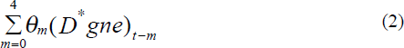
The dummy variable, D*, took the value unity during the period March 1990 until September 1991. The inclusion of these terms had little impact on the other estimates. Nevertheless, these slope dummies were jointly significant (p-value = 0.00), and the p-value for the test of significance of the original gne terms rose from 0.13 to 0.75. In other words, almost all of the explanatory power of gne comes from the recent recession.
This suggests that the shock in 1986 set the stage for the subsequent recession having an impact on exports. Up until that time, PW−PL was in a band of inaction. Nevertheless, in the sunk cost model, the subsequent recovery need not act to reduce exports.
Footnotes
Dwyer, Kent and Pease (1993) argue that export price pass-through is not as rapid for manufactures as it is for commodities. Nevertheless, to whatever extent an exchange rate depreciation causes a decline in the foreign currency price of Australian manufactures, the demand for exports should increase. In this case hysteresis may occur because the increased demand enables sunk costs to be covered. [22]
Sunk costs issues aside, gradual tariff reductions could also exhibit a sudden effect if, at some indefinable point, they came to be regarded as permanent. [23]
Consequently, the most established body of empirical literature on trade flows is that relating to single equation models of import demand. In contrast, modelling of exports is less established, Key examples of the literature on export models are Leamer and Stern (1970), Goldstein and Khan (1978) and, with respect to Australia, Ryder and Upcher (1990). [24]
Baldwin (1988) infers hysteresis from a structural break in an import equation, while Dixit (1989) discusses hysteresis using a model with imposed parameter values. [25]
The export revenue range was chosen to be comparable with the McKinsey and Co. (1992) study. See Appendix B. [26]
Some of the firms on the database did not export manufactured goods and some had ceased exporting. A preliminary screening question enabled those firms to be excluded from the sample. Furthermore, firms were also excluded when the first word of their name described their business (e.g. ‘Agribusiness’) and therefore determined their alphabetical order. [27]
It is reasonable to assume that companies' costs are totally unrelated to their order in the alphabetical listing. Also, it has also been argued that the characteristics of NSW exporting firms can be generalized to Australian firms (Daly et al. 1992). Companies consent to being on the AUSTRADE database because they have asked for assistance, to be informed of seminars or to be matched with buyers in overseas markets. A self selection problem may arise if only those companies with large sunk costs approach AUSTRADE. On the other hand, the fact that AUSTRADE has paid some of their sunk costs may mean that they do not realize the magnitude of them. It was usually necessary to contact Managing Directors or Financial Controllers and this meant that many of the interviews were conducted under time constraints. Anticipating this problem, an abbreviated version of the survey was offered to executives if they were too busy (questions 3 to 12 inclusive). This proved effective in raising the response rate. [28]
Of the 25 firms answering the relevant question, 2 stated that other firms had made their entry easier and 2 claimed to have made subsequent entry by their competitors easier. [29]
‘Significant’ means that the cost was taken note of when firms were considering an export venture. In describing the costs as sunk, it is implicitly assumed that they cannot be recouped if the firm exits the market. [30]
If capital is rented, then the costs are fixed rather than sunk. However, survey respondents indicated that their spending on these items declined once they had established themselves in a foreign market. The survey did not explore the issue of how saleable capital was in the event of exit. [31]
12 respondents indicated this out of 20 who answered the relevant question. [32]
Firms indicated the year in which they exported more than 10 per cent of their output. In a study by McKinsey and Co. (1992), 1986 was also highlighted as a significant entry year. [33]
It was confirmed that the 1986 observation did, in fact, reflect an increase in export volumes. All firms which nominated that year were contacted again to make sure that the increased share represented an increase in actual merchandise. [34]
25 exporters answered the question about the effects of the ‘recent recession’ and 20 answered the question about the effects of ‘any other recession’. With regard to the 1982/83 recession, 9 firms first exported more than 10 per cent of their production prior to 1983. Of these, 2 increased their exports in response to the recent recession and 1 of those 2 increased its exports in response to ‘another recession’ (probably 1982/83). Of the firms which indicated that they were exporting less than 10 per cent of sales in 1982/83, 2 said that the incentive to export was greater in the recent recession than it was in 1982/83. [35]
The construction and interpretation of this series is described in Appendix D. It is measured as a proportion; that is, 20 per cent is 0.2. [36]
This is because their share of Australia's exports has been rising recently. [37]
The estimation technique was OLS with a Newey-West correction for a nonscalar identity covariance matrix. Serial correlation was present, which implies inconsistent estimates, given the lagged dependent variable. The equation was estimated using IV with the broken trend as an instrument for x. The main result, namely that gne was insignificant and the broken trend was significant, was verified. A cointegrating relationship was found between exports and its explanators (excluding gne). Nevertheless, in order to verify the main result, the model was run in a difference form. Again gne was insignificant while the dummy was significant. [38]
This elasticity is defined as the per cent increase in exports resulting from a one percentage point increase in the effective rate of assistance to manufacturers. [39]
An alternative is that tariffs really do explain all the growth in the late 1980s. If this is so, then a strong tariff effect on imports should also be observable. [40]
This is true if exports are already occurring. [41]
Despite this, bands of inaction do not always imply the possibility of hysteresis. A band of inaction may exist if C is incurred each period. The survey is relied upon to establish that some costs are sunk. Given this, bands of inaction do imply the possibility of hysteresis. [42]
If a small proportion of manufactured output was sold domestically, it could be empirically difficult to find a significant relationship between exports and domestic demand. As it is, 70 per cent of manufactured output is sold domestically. [43]
In part, models with significant structural breaks were preferred to other models in the estimation process. The late 1980s surge in exports resulted in the estimated equations having either a significant structural break or, in a few versions of the model, very high exchange rate elasticities. Believing the latter result implied that exports were ‘explosive’. See Appendix C. [44]
There is very strong evidence that the series is ‘explosive’ unless there is a structural break. That is, the effects of an innovation to exports will magnify through time rather than die down. As this is highly implausible for an economic time series, the few versions of the model which did not have a significant structural break were abandoned. See Appendix C. [45]
While the late 1980s surge is modelled as a broken trend, it is not anticipated that recent rates of growth will continue indefinitely after the effects of hysteretic shocks, tariff reductions and vanguards have run their course. [46]