RDP 2025-07: Back to the Futures: Liquidity in Australian Bond Futures amid Market-moving Events since COVID-19 5. Effects of Regular Events on Liquidity
October 2025
We now turn to the effects of market-moving events that occur fairly regularly in our sample – specifically, RBA policy decisions, major economic data releases from the ABS, RBA bond purchases, AOFM bond sales and changes in minimum price increments, in particular in futures roll periods – on our measures of futures market liquidity. For regular events, we can estimate their effects with greater confidence than we can for one-off periods of interest. To do this, we compare liquidity on event days with uneventful ‘control’ days throughout our sample. We use our full sample from October 2019 to June 2025 for our estimations throughout Section 5, though a sample that excludes 2020, thereby excluding the period most affected by COVID-19, produces qualitatively similar results.
5.1 News events: RBA policy decisions and ABS data releases[15]
First, we estimate the effects of the RBA's monetary policy decisions and major ABS data releases. For each liquidity measure and futures tenor, we use an ordinary least squares regression (OLS) to estimate the following equation for the two types of news event separately:
where yd,t is the measure at time t on date d and xd is a binary treatment variable, indicating whether the news event occurred on that date (= 1) or not (= 0). We include fixed effects for dates and times of day . We cluster errors by date and time of day. Our sample consists of dates where that type of news event occurred and control dates, and excludes dates where other types of events occurred. Our control dates are Tuesdays where no market-moving events occurred. Given this, our coefficients of interest are , which can be interpreted as the average time-of-day effects for that type of news event relative to control dates and an arbitrary time (t0) prior to when the news event occurs.
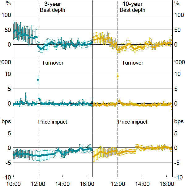
Figures 9 to 12 show model results in graphical form, where for each 5-minute increment the dot represents the mean effect of the news event on the given measure of liquidity in that 5-minute period and the whiskers show the 90 per cent confidence interval around that mean. Qualitatively, the results follow the same patterns as some of the events discussed in the previous section – bid-ask spreads increase, market depth falls, and price impact tends to rise, all indicative of a worsening in liquidity. Also similar to above, turnover rises despite the worse liquidity conditions, as investors adjust their portfolios following the news.
Beginning with bid-ask spreads in Figure 9, news events see a widening in the minutes leading up to the release, with spreads increasing by around 0.05 to 0.15 basis points, compared with a median bid-ask spread of 0.5 basis points. Liaison with market participants suggests that many liquidity providers, particularly those that utilise algorithms to make the market, pull back ahead of information releases, which may explain this pattern; this is also relevant for depth and price impact, as discussed below.[16] The effect is generally small and short-lived, however; for both the 3-year and 10-year contracts, spreads return to typical levels within around half an hour after the news event for RBA decisions, and within a few minutes for ABS data releases. The more rapid normalisation following ABS data releases, versus RBA decisions, is also apparent in the other liquidity metrics, and may indicate that the market is able to interpret ABS releases quickly, whereas it takes longer to fully interpret and price the new information contained in RBA decisions (including because RBA decisions are followed by a press conference for part of our sample).
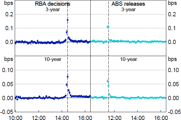
Notes: Whiskers show 90 per cent confidence intervals. X-axis shows the time of day in Sydney, from 10:00 to 16:25.
Sources: Authors’ calculations; Bloomberg.
Market depth in Figure 10 displays a pronounced and relatively longer-lived reaction to news events, and especially to RBA policy decisions. Depth falls by around 75 per cent at peak for RBA policy decisions for both the 3-year and 10-year contracts, and is materially lower than is typical for around 30 minutes either side of the event. For ABS data releases the response is similar but less pronounced, with depth falling by around 50 per cent for both the 3-year and 10-year contracts and remaining materially lower for 10 to 20 minutes either side of the event.
Conversely, turnover as shown in Figure 11 increases disproportionately after the event (versus before for the other measures), and it increases despite the less favourable liquidity conditions, as market participants observe and then trade on the news to rebalance their portfolios. For RBA policy decisions, turnover increases by around 7,000 and 3,500 contracts respectively for the 3-year and 10-year contracts – to a level around eight and five times typical turnover, respectively – and remains elevated through to the close of the day session. Again, for ABS data releases the response is similar but a little less pronounced.
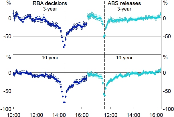
Notes: Whiskers show 90 per cent confidence intervals. X-axis shows the time of day in Sydney, from 10:00 to 16:25.
Sources: Authors' calculations; Bloomberg.
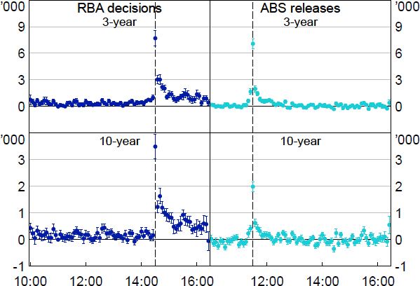
Notes: Whiskers show 90 per cent confidence intervals. X-axis shows the time of day in Sydney, from 10:00 to 16:25.
Sources: Authors' calculations; Bloomberg.
Finally, price impact as shown in Figure 12 tends to increase following news events, particularly for the 10-year contract, which is indicative of worse liquidity conditions. Recall that the price impact measure is estimated over a trailing 90-minute window excluding data 5 minutes either side of the news event; this means that by construction it has a high degree of persistence.
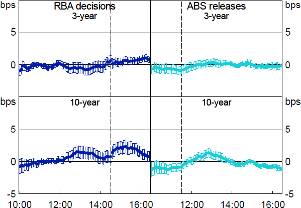
Notes: Whiskers show 90 per cent confidence intervals. X-axis shows the time of day in Sydney, from 10:00 to 16:25.
Sources: Authors’ calculations; Bloomberg.
5.2 Flow events: RBA purchases and AOFM tenders[17]
Large scheduled flow events – bond sales by the AOFM or purchases by the RBA – serve as a focal point for market participants, bringing investor attention, and therefore liquidity, to the market. We analyse flow events similarly to news events, but we replace the binary treatment variable with a continuous treatment variable representing the size of the flow, adjusted to apportion it between the 3- and 10-year futures contracts.[18] For example, for a tender of $1 billion of a 6.5-year bond, the continuous treatment variable would be $0.5 billion in each of the 3- and 10-year regressions. If the bond had 3 years to maturity instead, then the treatment variable would be $1 billion in the 3-year regression and zero in the 10-year regression (effectively, it would count as a control day in the latter regression). This approach approximates how market participants use a combination of 3-year and 10-year futures positions to hedge bond purchases. We do not report bid-ask spreads as they display minimal reaction to flow events.
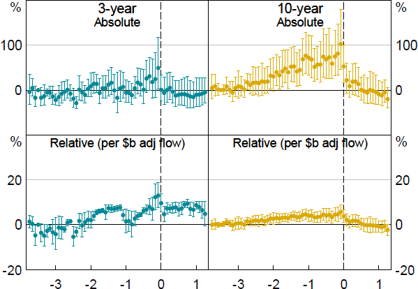
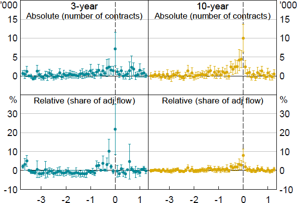
Figure 13 shows the effect on turnover from RBA purchases and AOFM tenders, expressed as a share of the adjusted flow amount. So, for example, if the purchase or tender flow apportioned to the 3-year contract was $1 billion, a 10 per cent effect size would mean that turnover in the 3-year contract rose by 1,000 contracts, equivalent to $100 million face value of bonds (i.e. 10 per cent of $1 billion) relative to control days in the relevant 5-minute window. As might be expected, turnover is elevated in the event window, with the magnitude of the increase around 10 to 20 per cent of the adjusted flow level; turnover is also elevated, but to a lesser extent, for 5 to 10 minutes either side of the event.[19] Flows are fairly evenly balanced between the buyer-initiated and seller-initiated sides for both event types.
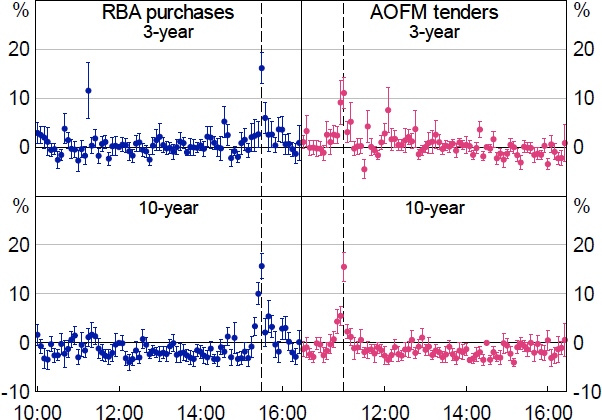
Notes: Whiskers show 90 per cent confidence intervals. X-axis shows the time of day in Sydney, from 10:00 to 16:25.
Sources: Authors’ calculations; Bloomberg.
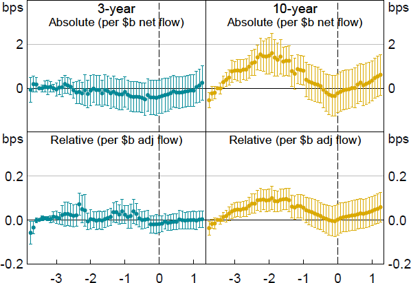
Figure 14 shows the effect on depth from RBA purchases and AOFM tenders. RBA bond purchases and AOFM bond tenders both result in modestly increased market depth for the hour or so leading up to the event, in the order of around 10 to 30 per cent per $1 billion of adjusted flow. The increase in depth around RBA purchases occurs on the bid side of the order book, whereas the increase around AOFM tenders is on the ask side; this is consistent with participants laying orders to hedge expected flows pre-emptively.
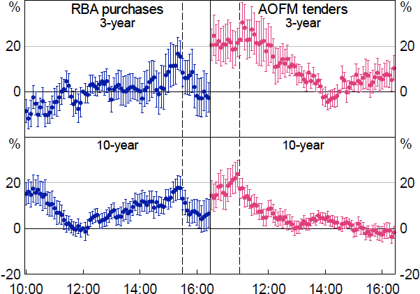
Notes: Whiskers show 90 per cent confidence intervals. X-axis shows the time of day in Sydney, from 10:00 to 16:25.
Sources: Authors’ calculations; Bloomberg.
Consistent with greater depth, price impact is typically little changed to modestly lower around these events (Figure 15).
Taken together, the above results suggest that RBA bond purchase and AOFM bond tender events improved liquidity conditions somewhat. These flow events – which are announced in advance – serve as a focal point and draw participants into the market, where they meet and transfer risk, which appears to improve liquidity for a short period. Each of the events represents a significant transfer of interest rate risk between the public and private sectors; if investors found it difficult to smoothly absorb that transfer, then this could result in worse or little changed liquidity conditions, though our findings suggest that this is not what occurs in the AGS futures market typically.[20]
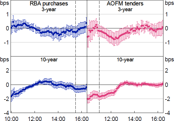
Notes: Whiskers show 90 per cent confidence intervals. X-axis shows the time of day in Sydney, from 10:00 to 16:25.
Sources: Authors’ calculations; Bloomberg.
5.3 Syndication events
AOFM syndications are the largest flows that the Australian Government bond market needs to absorb.[21] They are typically more than $10 billion in size, equivalent to 100,000 futures contracts. While issuance is on an outright basis from the AOFM's perspective (unlike other issuers that sometimes issue on a hedged basis using futures), AOFM syndications nevertheless involve a substantial volume of futures trades and have a major effect on the AGS futures market. First, around one-half of investors in a syndication typically submit orders for hedged bond purchases (known as ‘exchange for physical’, or EFP, in the market). These orders involve the hedge risk manager – one of the commercial banks that is involved in organising the syndication – executing short futures trades that hedge the interest rate risk of the bonds for the investor. The investor then receives the long bond position, plus an offsetting short futures position, when they take delivery of the bonds. The hedge risk manager will typically execute most, but not all, of the short futures trades ahead of syndication pricing, with the remainder executed over the course of the day. While the hedge risk manager bears the risk of moves in futures prices between execution and the pricing of the syndication, they spread out the flow to reduce the volume of short futures trades that must be absorbed by the market in a short period of time, as a concentrated flow close to the time of the syndication pricing could itself move futures prices. Second, some investors who purchase bonds outright (rather than EFP) will hedge the interest rate risk themselves, rather than via the hedge risk manager.
AOFM syndications tend to occur at longer tenors of 10 years or more (although there were three syndications for bonds with tenors of around 5 years in 2020), so we focus on 10-year futures in our discussion of estimated effects. For each liquidity measure and futures tenor, we use OLS to estimate the following equation:
where ys,d is the average measure for syndication s on day d, where d measures days relative to when that syndication was priced taking integer values between −7 and 4. We include fixed effects for each syndication and control for event types e occurring in the syndication period through binary variables ce,s,d, which cover the news and flow events analysed above, the futures contract roll periods analysed below, and the releases of RBA minutes and Reserve Bank of New Zealand (RBNZ) policy decisions, which take place during the Australian trading day and can move pricing for AGS futures. Errors are clustered by syndication. We scale the effects by the syndication amount, adjusted for the tenor of the syndication similarly to how we analyse the other flow events, through the continuous treatment variable xs. Our coefficients of interest are , which can be interpreted as the average day effects for syndications relative to an arbitrary day (d0) prior to the syndication period, set to be seven days before the pricing date. There are relatively few data points in general, and even fewer that are relevant for 3-year futures, because syndications occur infrequently.
Consistent with our analysis of smaller flows above, syndications tend to improve liquidity conditions on the day that they occur (Figure 16). Focusing on the 10-year contract, market depth rises by close to 10 per cent per $1 billion of adjusted flow (so a $10 billion 10-year syndication leads to a near doubling in depth). Turnover rises by roughly the same magnitude as the size of the syndication. The increases in depth and turnover occur on both sides of the order book, though for depth the increase on the ask side is somewhat more pronounced, in line with our finding for AOFM tenders. Price impact is substantially lower, by around 0.3 basis points per $1 billion of adjusted flow (so a $10 billion 10-year syndication would reduce price impact by around 3 basis points). We find broadly similar effects for the 3-year contract, but as there were only three syndications of shorter-dated bonds in our sample confidence intervals are wide and we do not focus on them.
Again, in theory large syndications could worsen liquidity, which would be the case if investors had trouble smoothly absorbing the additional interest rate risk sold to the market. That this is not the case suggests that the AGS futures market is deep and liquid enough to be able to smoothly absorb even very large flows. Indeed, large flow events serve as a focal point, bringing investors to the market to such an extent that liquidity is improved.
Notes: Whiskers show 90 per cent confidence intervals. X-axis shows days relative to the pricing day. Effects on turnover are shown as a share of adjusted flow. Effects on best depth and price impact are shown in per cent and basis points per $1 billion of net flow, respectively, with each expressed per $1 billion of adjusted flow.
Sources: Authors’ calculations; Bloomberg.
5.3.1 Announcements[22]
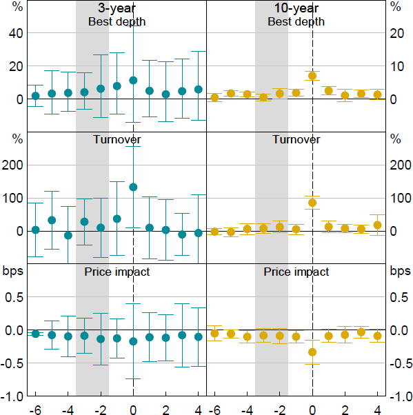
Syndications are officially announced a few days before they are priced, though the announcements are to some extent anticipated by market participants. For example, market participants may be fairly certain that a syndication will occur in a given month, most likely on one of a handful of days, but still be uncertain as to the exact day. We analyse announcement day effects similarly to other intraday effects. However, as the sample is substantially smaller for syndications, we do not filter out days where they clash with other events, whereas for our analysis of other events we do filter out these clashes. Most syndication announcements in our sample occurred on AOFM tender days. For reference, most announcements occurred on days –2 and –3 of the regressions displayed in Figure 16.
We find that intraday depth is elevated ahead of syndication announcements – likely due to announcements falling on AOFM tender days, which tend to be associated with greater depth – but that depth falls following the announcement, before returning to normal levels by the end of the day, as shown in Figure 17. Turnover spikes higher on the announcement, but the effect is very short-lived and turnover returns to pre-announcement levels within 5 to 10 minutes. And price impact is a little lower through most of the day, again most likely due to announcements falling on tender days. On net, and similar to news events, it seems that syndication announcements temporarily worsen liquidity conditions.
Notes: Whiskers show 90 per cent confidence intervals. X-axis shows the time of day in Sydney, from 10:00 to 16:25. Effects on turnover are shown in thousands of contracts. Effects on price impact are shown in basis points per $1 billion of net flow.
Sources: Authors’ calculations; Bloomberg.
5.3.2 Pricing days[23]
We cannot analyse pricing day effects exactly like other intraday effects since syndications are priced at different times in the afternoon on pricing days, ranging from around 13:45 to 15:15. Instead, for each liquidity measure and futures tenor, we use OLS to estimate the following equation:
where yd,t,r is the measure on date d at time t, and r is the time relative to the pricing time on syndication dates (on other dates r is irrelevant, as it is multiplied by the treatment variable xd, which is zero on other dates). For xd, we use either a binary variable (as we used for news events) or a continuous variable representing the adjusted flow from the syndication for each futures tenor (as we used for flow events). We include fixed effects for dates and times of day , and cluster errors by date and time of day. Our sample consists of syndication pricing dates and control dates but, just as for analysing syndication announcements, we do not exclude syndication pricing dates where other types of events occurred. Given this, our coefficients of interest are , which can be interpreted as the average relative-time-of-day effects for syndication pricings compared to our control dates and an arbitrary time relative to the pricing time (r0). For reference, pricing occurs on day 0 of the regressions displayed in Figure 16.
Figure 18 shows the results for market depth, with the top panels coming from a regression where the treatment variable is binary (pricing day or not), and the bottom panels coming from a regression where the treatment variable is continuous (being the dollar amount of syndication flow apportioned to the 3-year or 10-year contract). For both regressions and both contracts, depth rises in the few hours leading up to the pricing time. The effect size is large – peak depth is double the typical level for the 10-year contract, and around 50 per cent higher than typical for the 3-year contract. Similar to our finding for the increase in depth on the pricing day, the increase within the pricing day is also fairly balanced between the bid and ask sides of the order book, though slightly larger on the ask side. Depth returns toward more typical values soon after pricing.
Turnover also rises significantly around pricing, and for the 10-year contract is elevated for a short period before pricing, as shown in Figure 19. Focusing on the top-right panel, turnover in the 10-year contract rises by around 10,000 contracts in the 5-minute window containing the pricing time, versus median turnover of around 420 contracts per 5-minute window. This is unsurprising given that the hedge risk manager will be executing futures trades in the lead-up to and around the pricing time.
Notes: Whiskers show 90 per cent confidence intervals. X-axis shows time in hours relative to the pricing time, from –3:45 to 1:15.
Sources: Authors’ calculations; Bloomberg.
Notes: Whiskers show 90 per cent confidence intervals. X-axis shows time in hours relative to the pricing time, from –3:45 to 1:15.
Sources: Authors’ calculations; Bloomberg.
Figure 20 shows price impact on pricing days, with the top panels again coming from a regression where the treatment variable is binary (pricing day or not), and the bottom panels coming from a regression where the treatment variable is continuous (being the dollar amount of syndication flow apportioned to the 3-year or 10-year contract). For 10-year futures, the magnitude of the effects in the top panel are around 10 times the size of those in the bottom panel since syndications are typically around $10 billion in size and tend to be at longer tenors (i.e. the treatment variable is ‘1’ in the top panel regressions, and around ‘10’ in the bottom panel regressions). Despite higher depth, price impact tends to increase ahead of pricing, indicative of worse liquidity conditions. This is a period when the AOFM's hedge risk manager may be expected to be active in the futures market. Other market participants, knowing that the hedge risk manager is likely to need to transact a substantial quantity of futures contracts, may speculate around this activity, contributing to a more one-sided market and increasing price impact. Market contacts have also confirmed some deterioration in liquidity ahead of pricing. Recall, however, that these are intraday effects, controlling for the fact that the day is a syndication day. As discussed above and shown in Figure 16, price impact falls overall on syndication days, and the results of this section suggest that that fall is most pronounced at the time of pricing itself, which serves as a focal point for market participants to transact and transfer risk.
Notes: Whiskers show 90 per cent confidence intervals. X-axis shows time in hours relative to the pricing time, from –3:45 to 1:15.
Sources: Authors’ calculations; Bloomberg.
5.4 Increment events
Futures rolls are a major event in the futures market. Futures contracts expire on the 15th day of March, June, September, and December, or on the following business day if the 15th is a weekend or other non-trading day. Outside of roll periods, the overwhelming majority of trading activity occurs in the so-called front futures contract, that is, the contract closest to expiry. But the front contract expires every three months, and investors who wish to maintain their futures position post-expiry have to ‘roll’ from the expiring contract to the next contract. They do this by closing out their position in the expiring contract (e.g. selling futures if they are long) and entering a new position in the next contract (e.g. purchasing futures if they were long), usually in a single linked trade. Roll activity is concentrated in the five days leading up to expiry, and over this period the ASX typically narrows the minimum price increment that the futures contract can trade in, in order to make rolling positions less costly. Outside of the roll period, in October 2022 the ASX widened the minimum price increment for the 3-year contract, to try to improve liquidity in that contract.
A priori it is unclear what the net liquidity effect of changes in minimum price increments should be. On the one hand, wider increments make it more profitable for market makers to provide liquidity, and so should draw in more market making resources and thereby improve liquidity conditions. However, conversely, wider increments make it more costly for investors and arbitragers to trade, so could drive away users of the product. The net effect may depend on starting liquidity conditions: in a very liquid market, narrow increments should help to attract investors and arbitragers, and high trading volumes should make intermediating the market profitable to market makers, even with narrow bid-ask spreads; this scenario appears to accord with the findings of Fleming et al (2024) regarding the US Treasury market. In a less liquid market with lower trading volumes, market makers may need wider bid-ask spreads to incentivise them to provide intermediation services. The dependence of the net effect of tick size changes on starting liquidity conditions is consistent with the model and empirical evidence presented in Werner et al (2023), who examine equity exchanges in the United States and Japan.
5.4.1 Increment changes during and between futures roll periods
We analyse futures roll periods similarly to syndication periods, with a few adjustments: the treatment variable is set equal to 1 (as, unlike for syndication periods, there is no need to scale the effects for roll periods); the reference day d0 is set to be nine days before the expiry day, which day d is relative to; and roll periods are excluded from the controls whereas syndication announcement and pricing dates are included.
Figure 21 shows estimated effects on bid-ask spreads and best depth for the 3-year futures contract from four distinct samples:
- ‘pre-narrowing’, which covers December 2019 and March and June 2020, where the minimum price increment during the roll period was equal to the normal increment of 0.5 basis points.
- ‘post-narrowing’, which covers September 2020 to September 2022, where the minimum price increment was reduced from 0.5 to 0.2 basis points during the roll period.
- ‘post-widening’, which covers December 2022 to December 2024, where the minimum price increment was reduced from 1 to 0.2 basis points during the roll period (as the normal increment was increased from 0.5 to 1 basis point in October 2022, which we analyse further below).[24]
- ‘post-delinking’, which covers March and June 2025, where trading in the roll and outright futures markets were delinked, so that the minimum price increment for outright futures trading remained at 1 basis point despite the roll trading in 0.2 basis point increments.
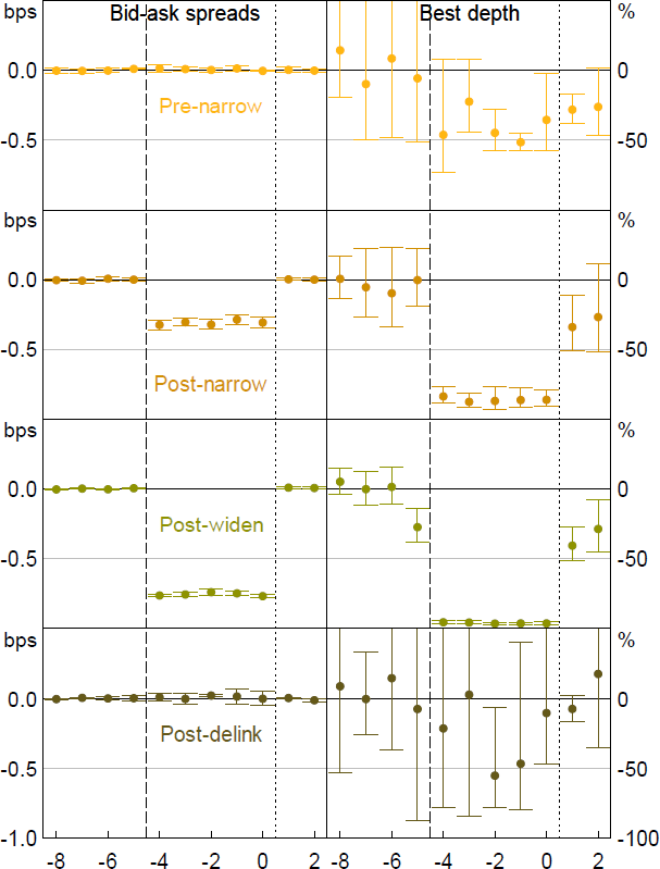
Notes: Whiskers show 80 per cent confidence intervals. X-axis shows days relative to the expiry day. Some confidence intervals for best depth are truncated.
Sources: Authors’ calculations; Bloomberg.
These adjustments are clearly visible in the top panel of Figure 3, which shows no change in average bid-ask spreads around rolls initially, then periodic dips from 0.5 to 0.2 basis points, then a step-up in the general level of bid-ask spreads but no change in the level during rolls, and finally no change around rolls once again, though now at a higher level. Note that the pre-narrowing sample contains just three episodes, and the post-delinking sample just two episodes, so the confidence intervals for these samples tend to be wider than for the other two samples.
The four left panels of Figure 21 show the estimated effects on bid-ask spreads. As noted earlier, bid-ask spreads are usually very close to the minimum price increment, and this is typically the case during roll periods too (other than for the front contract on expiry day and the day before). This results in estimated effects on bid-ask spreads from pre-roll to the roll period of close to 0, 0.3, 0.8 and 0 basis points, respectively, for the four samples just described, that is, equal to the change in minimum price increment.
Table 1 presents analogous results from a local randomisation approach within a simple regression discontinuity design, which uses the five days immediately prior to the beginning of the roll period as the control (rather than the single day five days before the roll period begins), and estimates a single treatment effect for the whole roll period (rather than a different treatment effect for each day within the roll period).[25] This approach again finds falls in bid-ask spreads of close to the change in minimum price increments across the four samples.
| 3-year futures contracts | 10-year futures contracts | |||||||
|---|---|---|---|---|---|---|---|---|
| Pre-narrowing | Post-narrowing | Post-widening | Post-delinking | Pre-narrowing | Post-narrowing | Post-delinking | ||
| Bid-ask spreads (basis points) | 0.0 (0.0, 0.0) |
−0.3*** (−0.4, −0.3) |
−0.8*** (−0.9, −0.6) |
0.0 (0.0, 0.0) |
−0.2*** (−0.3, −0.2) |
−0.4*** (−0.4, −0.3) |
0.0 (0.0, 0.0) |
|
| Best depth (per cent) |
−34 (−71, 42) |
−83*** (−91, −69) |
−96*** (−98, −93) |
−31** (−46, −12) |
−74*** (−85, −55) |
−95*** (−96, −92) |
−31** (−46, −14) |
|
| Turnover (‘000s of contracts) |
−24* (−46, −3) |
−19*** (−27, −11) |
−31*** (−41, −20) |
−38** (−65, −11) |
−19 (−42, 2) |
−42*** (−49, −34) |
−27 (−55, 0) |
|
| Price impact (basis points per $b of net flow) |
2.0** (0.3, 3.7) |
1.7* (0.1, 3.4) |
3.4*** (2.5, 4.4) |
1.1* (0.0, 2.2) |
4.5*** (1.8, 7.4) |
6.3*** (4.8, 7.8) |
1.9*** (0.7, 3.2) |
|
|
Notes: *, ** and *** denote statistical significance at the 10, 5 and 1 per cent levels, respectively. Parentheses show bootstrapped 90 per cent confidence intervals. Sources: Authors’ calculations; Bloomberg. |
||||||||
The four right panels of Figure 21 show the estimated effects on best depth for the 3-year contract. One might expect depth at the best available price to fall as the minimum price increment narrows. For example, in the post-narrowing sample, bids within a single 0.5 basis point increment prior to the roll could now be spread over 2½ smaller 0.2 basis point increments during the roll. And this is indeed what we see, in both Figure 21 and in the local randomisation estimates shown in Table 1. But depth falls by more than might be expected naively if the minimum increment was the only explanation, assuming that orders would be layered uniformly between price increments were that possible. For example, during the roll period, depth falls by:
- around 85 per cent in the post-narrowing sample whereas a 60 per cent fall would be more in line with the change in minimum price increment.
- around 95 per cent in the post-widening sample whereas an 80 per cent fall would be more in line with the change in minimum price increment.
Additionally, based on the estimates in Table 1, depth falls by around one-third in the pre-narrowing and post-delinking samples where bid-ask spreads are unchanged, though the estimate for the former sample lacks statistical significance. Underlying turnover, shown in Table 1, also tends to fall during the roll period. This excludes trades associated with the roll itself, which inflate turnover substantially.
Thus, the roll period itself seems to result in less depth, not just the mechanical change in minimum price increment (when such a change occurs). This conclusion is supported by the bottom row of Table 1, which shows that the estimated price impact of trades increases by a few basis points during the roll period, indicating that the roll is associated with worse liquidity conditions than normal. Two potential explanations for this include that:
- the roll diverts investors’ and dealers’ attention and resources from the outright market, and so results in worse liquidity conditions for a period
- the narrower minimum price increment (when implemented) – and therefore lower bid-ask spread – means that market makers earn less from intermediating trades and so devote fewer resources to that activity, in terms of their balance sheet capacity, resulting in worse liquidity conditions.
Liaison with market participants suggests that both explanations are to some extent true, with the latter explanation noted as applying in particular for algorithmic market makers.
Figure 22 shows the same as Figure 21 but for the 10-year contract, for which there is no distinct post-widening sample. In the pre-narrowing sample, the minimum price increment during the roll period falls from 0.5 basis points to 0.25 basis points. In the post-narrowing sample, covering September 2020 to December 2024, the minimum price increment during the roll period falls from 0.5 basis points to 0.1 basis point. In the post-delinking sample, the minimum price increment for outright futures trading remained at 0.5 basis points during the roll despite the roll trading in 0.1 basis point increments. These adjustments are clearly visible in the top panel of Figure 4. Again, the pre-narrowing sample contains just three episodes, and the post-delinking sample just two, so confidence intervals for these samples tend to be wider than for the other sample. As before, Table 1 contains analogous results from a local randomisation approach.
Overall, the pattern of results is very similar to the 3-year contract: the bid-ask spread falls by roughly the same magnitude as the change in minimum price increment across the three samples (being 0.25, 0.4 and 0 basis points respectively); market depth falls, and more so than might be expected given the mechanical effect of a smaller minimum price increment (by around 75 per cent in the pre-narrowing sample, whereas 50 per cent might be expected; by around 95 per cent in the post-narrowing sample, whereas 80 per cent might be expected; and by around one-third in the post-delinking sample despite no change in the tick size); price impact increases; and turnover falls. Again, these results suggest that the roll period results in worse liquidity conditions.
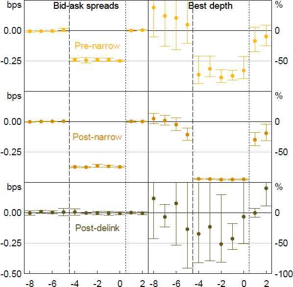
Notes: Whiskers show 80 per cent confidence intervals. X-axis shows days relative to the expiry day. Some confidence intervals for best depth are truncated.
Sources: Authors’ calculations; Bloomberg.
5.4.2 Increase in the minimum price increment for the 3-year futures contract
In October 2022, the ASX increased the minimum price increment that the 3-year futures contract could trade in, from 0.5 to 1 basis point, in an effort to improve liquidity conditions in that contract. Figure 23 shows daily measures of liquidity around the change, for both the 3-year contract, which experienced the change, and the 10-year contract, which saw no change in minimum price increment and so can act as a control. From a visual inspection, depth in the 3-year contract seems to have increased relative to depth in the 10-year contract, and price impact perhaps fell, while it is hard to discern a clear pattern in turnover.
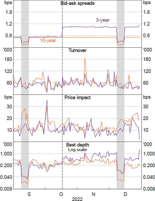
Notes: Best depth and turnover are shown in thousands of contracts. Price impact is shown in basis points per $1 billion of net flow.
Sources: Authors’ calculations; Bloomberg.
To formalise this visual analysis, we use a difference-in-differences approach with the 10-year contract as a never-treated control. That is, for each liquidity metric, we compare the difference between the 3-year and 10-year contract after the increase in minimum price increment to the difference between the two contracts before the increase in minimum price increment. The idea is that the 10-year contract will capture any market-wide impacts on liquidity, with the difference between the two contracts isolating events that only affect the 3-year contract. This implicitly assumes that there were no events affecting liquidity in the 10-year contract but not the 3-year contract, and that the only event affecting liquidity in the 3-year contract specifically was the increase in the minimum price increment. It is likely that liquidity in the 3-year futures contract (and 3-year AGS) was gradually improving over time, due to a policy of the AOFM to issue more 3-year bonds to support liquidity in that sector and the end of unconventional monetary policies by the RBA, among other things. In principle this would violate our assumptions, but in practice any improvement in liquidity due to these slow-moving factors, measured over a short period, is likely to be small in size.
More formally, for each liquidity measure, we use OLS to estimate the following equation:
where yc,d,t is the measure for contract c at time t on date d and pc,d is a binary post-treatment variable, indicating whether the contract was treated and the date is after the treatment (so pc,d equals one for 3-year futures starting from 18 October 2022, and zero otherwise). We include fixed effects for dates and times of day , and we cluster errors by date and time of day. We also control for event types e occurring in the period around the increment increase through binary variables xe,d, which cover the news and flow events analysed above, including syndication events, as well as RBNZ policy decisions and RBA minutes. Our coefficient of interest is , which can be interpreted as the aggregate average treatment effect on the treated for the period considered. We consider the full period between the September and December 2022 futures roll periods, and two shorter periods of ±20 and ±10 days around the increment increase.
In line with the visual inspection, we find that depth in the 3-year contract increased materially relative to depth in the 10-year contract following the increase in the minimum price increment (Table 2). While the magnitude of the increase in depth is around what one might mechanically expect following a doubling in increment size, the estimated fall in price impact after the increment increase suggests that the ASX's change improved liquidity conditions beyond the mechanical effect on depth (bottom row of Table 2). Turnover was little changed to slightly lower. Overall, a wider increment seems to have improved liquidity conditions in the 3-year futures contract, as was the ASX's intention in making the change.
| Full period between rolls | ± 20 days around increase | ± 10 days around increase | |
|---|---|---|---|
| Bid-ask spreads (basis points) |
0.5*** (0.0) |
0.5*** (0.0) |
0.5*** (0.0) |
| Best depth (per cent) |
94*** [84, 103] |
65*** [56, 74] |
71*** [60, 83] |
| Turnover (‘000s of contracts) |
−0.1* (0.0) |
0.0 (0.0) |
0.0 (0.1) |
| Price impact (basis points per $b of net flow) |
−2.8*** (0.5) |
−2.8*** (0.8) |
−3.0** (1.0) |
|
Notes: *, ** and *** denote statistical significance at the 10, 5 and 1 per cent levels, respectively. Parentheses show standard errors clustered by date and time of day; square brackets show an interval of ±1 standard error. Sources: Authors' calculations; Bloomberg. |
|||
Footnotes
In the regressions for this section, we drop the time-of-day fixed effect for 11:00 for RBA policy decisions, and 15:00 for ABS data releases. This allows us to include a date fixed effect and means that the measured effect at the relevant time (chosen to be several hours away from the event time) is zero. The ABS data releases we consider are: the quarterly consumer price index, national accounts and wage price index; and the monthly labour force survey and retail trade survey. [15]
Rapid price changes may also lead to wider bid-ask spreads, although this is more likely to be a factor after the data has been released, rather than before. [16]
In the regressions for this section, we drop the time-of-day fixed effect for 12:00 for RBA purchase days, and 14:30 for AOFM tender days. This allows us to include a day fixed effect and means that the measured effect at the relevant time (chosen to be several hours away from the event time) is zero. The RBA purchases we consider are purchases of AGS under the RBA's bond purchase program. For more information about the RBA's bond purchase program, see Finlay et al (2023). [17]
Other approaches to dealing with differences between the tenors of futures contracts and bonds bought or sold – for example, grouping bonds by the closest futures contract tenor rather than apportioning them between the contracts – produce qualitatively similar results. [18]
Notably, turnover is elevated for 3-year futures on RBA purchase days at 11:15, which is when the RBA would announce the bonds that would be eligible for purchase on those days, including any purchases of 3-year bonds to support the RBA's yield target. Turnover for 3-year futures at 11:15 was especially high on a number of days in September 2020 and February, March and October 2021, when participants expected the RBA to announce purchases of 3-year bonds to defend the target. For more information about the RBA's yield target purchases, see Finlay et al (2023). [19]
For comparison, Fullwood and Massacci (2018) find no discernible effect on liquidity dynamics around Bank of England asset purchase facility purchases in 2016; see their Figures 11 and 12, where higher numbers denote worse liquidity. [20]
Unlike tenders, where the AOFM ‘taps’ an existing bond line through an auction process, AOFM syndications typically involve the issuance of a new bond line, which is placed directly with investors with the support of a panel of commercial banks that organise the syndication. For more information, see AOFM (2019). [21]
In the regressions for this section, we drop the time-of-day fixed effect for 15:30. This allows us to include a day fixed effect and means that the measured effect at the relevant time (chosen to be several hours away from the event time) is zero. [22]
In the regressions for this section, we drop the fixed effect for the 5-minute interval that is 3.5 hours prior to the pricing time. This allows us to include a day fixed effect and means that the measured effect at the relevant time (chosen to be several hours away from the event time) is zero. [23]
Subsequently, in July 2025, the ASX reverted the normal increment for the 3-year futures contract to 0.5 basis points, though we do not analyse the effects of this increment change. [24]
No controls were used in this simple design. Consistent with the local randomisation approach, we use a uniform kernel and a polynomial of order 1. We use a 5-day bandwidth as this is supported by some bandwidth selection methods, but other bandwidths produce qualitatively similar results. [25]