Research Discussion Paper – RDP 2025-04 HANK and the Transmission of Shocks to Demand and Supply
June 2025
1. Introduction
In this paper, we study the importance of heterogeneity and individual microeconomic behaviour for aggregate outcomes in the Australian macroeconomy. Specifically, we make a first attempt at considering how differences in productivity and income across individuals in Australia can lead to differences in their decisions about consumption, savings, and working hours. Further, we explore how shocks to the economy impact different individuals in different ways, and how their reactions to these shocks may matter for the overall response of the economy.
Over recent decades, there's been an increasing realisation that distributional aspects can be important for the transmission of shocks to the economy, as well as the distributional impacts of policies and shocks. The heterogeneous agent New Keynesian (HANK) approach provides a powerful tool to better understand the transmission of policy at the household level by microfounding the optimal decisions of individuals with diverse outcomes. It allows for the understanding of how heterogeneity can change the the transmission of aggregate economic shocks, as well as how such shocks affect inequality (Acharya and Dogra 2018).
There are a number of channels through which a nontrivial distribution of income and wealth may affect shock transmission as compared to a world with a representative agent. For example, in a representative agent setting, all individuals are net savers, and will experience a fall in interest income and a rise in wage income in response to a fall in interest rates, with the net effect being an increase in consumption due to intertemporal substitution. In a heterogeneous agent setting, some households will be net savers while others will be net borrowers, and they will experience different effects on their income sources depending on where they land in the distribution. Depending on how a given household's current and expected future income is impacted, they may increase consumption in response to a rate cut while others may reduce it, with a similar response for labour hours and asset holdings. These variable responses could change the overall impact of the shock on the economy.
In turn, there are also channels through which the shock may affect the distribution of wealth. Leong (2021) highlights several possible channels through which monetary policy easing can affect wealth inequality. For example, there is the savings redistribution channel, whereby lower interest rates decrease fixed income returns and payments on debt, making borrowers better off and savers worse off. Similarly, there is the portfolio composition channel, wherein lower interest rates increase asset prices, possibly making the holders of these assets wealthier. While these channels suggest that policy shocks may have an impact on the wealth distribution, they likely act in the opposite direction for rate increases, suggesting that monetary policy may be neutral with respect to the distribution over the business cycle.
The primary aims of this paper are to examine the impact and transmission of aggregate economic shocks in a basic HANK model calibrated to the Australian economy. While much of the literature examines such models featuring multiple asset classes and unforeseeable economic shocks, in this work we consider a single asset, government bonds, which is closer in spirit to traditional representative agent New Keynesian (RANK) models. We do this as a first step towards building more sophisticated models for the Australian economy.
While this study is an important first step towards modelling the implications of heterogeneity for the transmission of shocks and conduct of monetary policy in Australia, these initial results are subject to a number of caveats. Shock transmission may be affected by the details of the composition of household assets and liabilities. This may be particularly important given the prevalence of less liquid assets such as housing and superannuation in Australia. Likewise, we do not consider secondary markets for bond assets in our economy, wherein nominal bond values could fluctuate for reasons other than interest rate changes. Moreover, we do not consider other aspects of heterogeneity which may be important for shock transmission, such as the life cycle or unemployment. Finally, in order to focus on realistic income and wealth dynamics without additional complications, the current study does not consider open economy dynamics. Further modelling in Australia will be needed to fill these gaps.
Having constructed the model, we proceed to describe various supply and demand shocks that could be considered in the model and compare the response of the heterogeneous agent economy to that of a representative agent counterpart. On the demand side, we consider a surprise decrease in the nominal interest rate (a monetary policy shock). We find that heterogeneity dampens the immediate real impacts of this shock, but slightly amplifies the inflation impacts. The dampened real response is in disagreement with much of the international literature on heterogeneous agent models, and likely reflects the lack of liquidity-constrained, high marginal propensity-to-consume households.
We then examine how household behaviour varies across the distribution of wealth in response to the monetary policy shock – by examining how the optimal consumption, work, and savings decisions adjust on impact. We find divergences in this behaviour across the distribution; for example, increased consumption by the middle quintiles of the wealth distribution is offset by those agents at the extremes. More specifically, the decline in interest rates results in a loss of income for very wealthy households who hold large stocks of liquid assets, causing these agents to cut consumption. On the other hand, the poorest households respond to a resulting increase in real wages by working longer hours, using the additional income to move away from the borrowing constraint. Correspondingly, we observe that the monetary policy easing generates a decline in wealth inequality in the model as measured by the Gini coefficient.
Next, we turn to shocks on the supply side of the economy. In particular, we consider two types of such shocks. First, we examine a shock to households' labour supply which increases their disutility from working. Second, we examine a shock to the substitutability between firm inputs (a mark-up shock). In the case of the former, we once again find considerable variation in behavioural adjustments across the wealth distribution, while in response to the latter we find much more homogeneity. This suggests that heterogeneity may be more important for shocks which directly impact the household optimisation problem. In both cases, we once again find dampened effects on the real economy.
The rest of the paper is organised as follows. Section 2 describes the literature. Section 3 outlines the model. Section 4 describes the data and calibration procedure, Section 5 outlines the shocks considered in the model, Section 6 presents our quantitative results, and Section 7 concludes.
2. Literature
The HANK literature has rapidly evolved in the past several years. This literature builds off of several decades of earlier work which weakened the complete markets hypothesis to consider a variety of questions in environments with heterogeneous outcomes. Early papers in this area, such as Bewley (1977), Aiyagari (1994) and Krusell and Smith (1998), laid the computational groundwork for solving them and studied foundational properties. Later work built on the computational tools (such as Reiter (2009)), and looked at a variety of applications (such as Heathcote (2005)). As computational methods improved, attention turned to the transmission of aggregate shocks in these models, including those due to monetary policy.
An influential piece of work which was one of the first to add New Keynesian price rigidities in a heterogeneous agent model was Kaplan, Moll and Violante (2018). Arguing that the proportion of households who are wealthy but hold exclusively illiquid assets is significant, the authors show that these wealthy hand-to-mouth households have a consumption response to interest rate changes that primarily arises from the impact of the change on their wage income (a general equilibrium effect). Simulating the HANK model by way of an MIT shock, they find that this effect outweighs the traditional intertemporal substitution effect in the model.
Prior to this work, Guvenen et al (2015) examined high quality administrative tax data from the Internal Revenue Service of the United States. Among other things, this work estimated several moments of the distribution of income changes. Kaplan et al (2018) then used these moments to calibrate the process for income in their model.
Alongside this work, Ahn et al (2018) introduced a continuous time variant of the method in Reiter (2009) for solving heterogeneous agent models. This method solves nonlinearly for the stationary equilibrium of the model, linearises the dynamic equilibrium conditions around the steady state values, and then solves the linear system. Ahn et al show that this method can solve baseline heterogeneous agent models much more efficiently than older methods, when the number of individual state variables is relatively small. As noted in the introduction, this is the solution method applied in this paper.
More recent developments in the broader HANK literature have explored the implications of heterogeneity for the exchange rate channel of monetary policy in small open economies (e.g. Auclert et al 2021) and the role of financial frictions and credit constraints in the HANK framework (e.g. Faccini et al 2024). The former paper finds that heterogeneity amplifies the extent to which a lower exchange rate reduces household real incomes and hence spending. This results in the potential for a currency depreciation to be contractionary, making expansionary monetary policy less expansionary. The latter paper finds that elevated credit spreads reduce consumption of indebted households in Danish data, resulting in a countercyclical propensity to consume. The authors calibrate a HANK model with financial frictions to match these observations, and conclude that regulatory measures may be stabilising at the aggregate level but volatility inducing at the household level. These are just two examples of questions being examined in a rapidly expanding body of literature.
As well, this paper is related to other papers exploring the differences between shock transmission in heterogeneous agent models and representative agent models. Kaplan and Violante (2018) show that responses to unforeseen shocks may differ or be similar between HANK and RANK, depending on the nature of the shock. They show that in response to a discount factor shock, the models have similar responses with similar underlying mechanisms, while in response to a technology shock they have similar aggregate responses but with different underlying mechanisms. They also show that monetary policy shocks generate different aggregate responses in HANK versus RANK. Finally, Kaplan and Violante highlight the fact that certain macroeconomic questions can only be addressed with heterogeneous agents, such as those on how a given shock affects individuals across the distribution.
Auclert, Rognlie and Straub (2020) study the transmission of monetary policy and sources of business cycle fluctuations in a HANK model. They find that investment plays a larger role in HANK relative to RANK. In particular, they find that if investment could not adjust in response to a policy shock, then the cumulative output response would be only 20 per cent of that when investment does adjust, in contrast to 60 per cent in RANK. They also find that matching a realistic distribution of marginal propensity to consumes (MPCs) in the model allows for procyclical co-movement of consumption and investment in response to an investment shock, offering a resolution of a puzzle dating back to Barro and King (1984), wherein RANK models require total productivity shocks for procyclicality.
While most of the HANK literature finds that household heterogeneity amplifies the effects of monetary policy, Cantore et al (2023) find a dampening effect on policy through the household labour supply channel. They provide some empirical evidence that following a contractionary monetary policy shock, lower income households tend to increase their hours worked. Building this added worker effect into a model they show that it can dampen the effects of monetary policy.
Guo et al (2023) measure the extent to which consumers face liquidity, savings, or borrowing constraints in data from 20 European countries. They consider whether the income and wealth distributions influence the effectiveness of tax and spending polices. The authors find that tax multipliers are amplified by a higher percentage of wealthy hand-to-mouth households, while spending multipliers are amplified by a higher percentage of poor hand-to-mouth households. They also find that a high proportion of wealthy hand-to-mouth households enhances monetary policy effectiveness, but a high proportion of households that are constrained in terms of liquidity, savings, and borrowings weakens it.
Overall, the literature on HANK models and supply and demand shocks highlights the importance of heterogeneity in understanding macroeconomic outcomes. In the existing body of research, HANK models have been employed extensively to analyse various economies around the globe. These models, with their inherent ability to capture economic realities more accurately due to their consideration of individual heterogeneity, have significantly contributed to our understanding of diverse economic phenomena.
Despite HANK models being adopted by academics and policy institutions internationally, there's a dearth of studies focusing on the Australian economy. This paper seeks to fill this gap in the literature by calibrating a HANK model to Australia and examining the implications for shock transmission relative to a representative agent framework.
3. Model
Broadly speaking, a HANK model is an economic model in which agents differ in some way (heterogeneous agents) and firms face frictions when they change prices (New Keynesian). The latter feature leads to a role for monetary policy. While a number of such models currently exist in the literature, in this paper we consider the simplest extension of a classical representative agent specification that is capable of generating a distribution of net worth similar to that of the Australian economy. We do this as a starting point to demonstrate the value of these models. In particular, we assume that households have access to a single savings vehicle, government bonds, with which to smooth consumption in response to aggregate shocks. This is the same assumption underlying the broader dynamic stochastic general equilibrium (DSGE) literature.
Time is continuous and infinite, and all agents are infinitely lived. The economy is populated by a unit measure of households who consume and work, and a unit measure of monopolistic goods firms who set prices to maximise profits. There is also a representative final good firm which combines output from the monopolistic firms into a final consumption bundle. The government adjusts lump sum transfers to stabilise debt, and the central bank sets the nominal interest rate in response to inflation. In the HANK model, however, households are unable to insure against their own individual productivity shocks, resulting in differences in income, consumption, and wealth.
In the remainder of this section, the precise optimisation problems solved by the individuals in the economy are described in greater detail. Specifically, we describe the objectives that they try to maximise, what constraints they are subject to, and the resulting optimal behaviour rules. These rules, taken together, characterise equilibrium in the economy.
3.1 Households
There is a unit measure of ex ante identical households who value consumption and dislike working. Given streams for consumption ct and hours worked nt, a household's expected lifetime utility is given by
where is the time rate of preference. Flow utility u takes the form
in which denotes constant relative risk aversion (CRRA), is the reciprocal of the Frisch elasticity of labour supply, and is the weight on disutility from working.
Households have access to a single asset, government bonds, with which to self-insure and hence smooth consumption and working hours. Denoting household bond holdings by bt, the time rate of change dbt/dt of these holdings is given by the household's income minus its expenditures on consumption. Income is derived from interest payments on current bond holdings, wages for hours worked, dividend payments derived from ownership of monopolistic firms, and lump sum government transfers. Interest income is given by Itbt, where It denotes the nominal interest rate. Wages are given by , where is the labour income tax rate, is the nominal wage rate, and zt is individual labour productivity. Denoting the real value of firm dividends by Dt and real lump sum transfers by Tt, then government bond holdings evolve according to
where Pt is the price of the consumption good and dividends are distributed independently of individual productivity or wealth. Defining the inflation rate as
it can be shown that this can be rewritten in real terms as
where is the real interest rate, Wt is real wages, and at = bt/Pt is the real value of government bond holdings. Households can borrow, but only up to some limit, so that bond holdings must satisfy
In the bond evolution equation (Equation (5)), households take the inflation rate, wage rate, dividends and transfers as given, while the labour income tax rate is fixed throughout time. Individual productivity, on the other hand, evolves according to an exogenous stochastic process. Specifically, we assume that productivity can take on J different states, with jumps between states j and j′ arriving according to a Poisson process with rate . Critically, due to the lack of a market for assets apart from government bonds, and in particular the lack of contingencies for productivity outcomes, households are unable to insure against their individual productivity risk. As a result, households in the model vary in income reflecting their productivity level, and consequently asset accumulation, resulting in a non-trivial equilibrium distribution of wealth.
The solution to the household problem is a process for consumption and hours which maximises Equation (1) subject to the Constraints (5) and (6). It can be shown that this problem can be rewritten recursively by defining the value function vt (a, z) as the maximum value of Equation (1) for a given level of bond holdings a and productivity state z. The solution is then given by behaviour rules ct (a, z) and nt (a, z) which decide consumption and hours for these levels of bond holdings and productivity, which in turn satisfy the Hamilton-Jacobi-Bellman equation
The first order conditions for the maximisation in this equation give the intertemporal smoothing motive,
expressing the trade-off between consumption now versus in the future, and the consumption leisure trade-off,
which reflects the disutility of working. Given the solution of the above equations for the consumption and labour rules, the distribution of wealth evolves from its initial state according to the associated optimal savings behaviour, in a manner dictated by the Kolmogorov forward equation
Here Ft denotes the probability density function of households over assets a and productivity states z, while st denotes the optimal time rate of savings of a household with asset holdings a in productivity state z. Thus the above equation expresses the change in the share of households in each state as the net flow of agents out of the wealth state while remaining in the same productivity state, combined with the flow of agents to new productivity states.
3.2 Firms
The supply side of the economy consists of monopolistic firms which produce individualised goods and a competitive sector which bundles these goods into a final consumption product. All firms are profit maximising. Workers are employed by monopolistic firms, who adjust their prices while incurring a cost for doing so via a Rotemberg rigidity. All profits from the sale of intermediate goods are paid as dividends to the households.
Specifically, the final goods firms choose how much of each intermediate product to include in the consumption basket, in order to minimise their costs while meeting demand, which they take as given. Given inputs , the amount of the final good produced is given by
where denotes the elasticity of substitution between inputs. Denoting the price of intermediate good j by pj,t, then these firms seek to minimise
subject to the constraint that the quantities of intermediate goods demanded sum to meet demand Yt :
It can be shown that the solution to this problem yields the demand schedule for intermediate goods,
and the zero profit condition then delivers the price level,
Monopolistic intermediate goods firms, on the other hand, take the demand schedule (Equation (14)) as given and hire labour nj,t to produce their individual products according to the technology
where Zt is total productivity common across all firms. These firms hire sufficiently to meet their demand, while minimising wage costs; however, due to there only being one factor of production, cost minimisation is trivial and the firms simply hire according to
The firm then chooses the price pj,t of its output to maximise expected discount future real profits, computed as revenue from sales minus wage and price adjustment costs
where and controls the magnitude of the cost to adjust prices. We consider a symmetric equilibrium in which all firms choose the same price every period. In this case, it can be shown that the solution of the firm's problems delivers a Phillips curve,
This is a similar condition to that in representative agent models, namely it relates inflation to firm marginal costs (wages) and expected future inflation.
3.3 Government
The government in the model economy taxes labour income and supplies bonds in order to finance its own expenditures, lump sum transfers to households, and interest payments on existing debt. In real terms, its budget identity is given by
where At is the real value of aggregate bonds outstanding, Gt is government expenditures, and Nt is aggregate efficiency hours. In order to stabilise the level of debt, transfers adjust to deviations of the debt away from its steady-state value according to
where variables without time subscripts denote steady-state values, controls the strength of the fiscal response to deviations of debt from target, and represents a fiscal shock.
3.4 Monetary policy
Monetary policy follows a Taylor rule in which the nominal interest rate responds to inflation according to
in which controls the central bank response to deviations of inflation from the steady-state value of zero, and represents a monetary policy shock.
3.5 Representative agent model
To draw out differences in shock transmission between HANK and RANK we consider an equivalent RANK model. The representative agent analogue of the model described in the previous sections is taken to be equivalent apart from the individual productivity process for households. In this version of the model, we assume that households have access to rich financial markets which allow them to insure against all idiosyncratic risk and hence receive the wages of an average worker every period. In this case, it can be shown that the household optimisation delivers as an equilibrium condition the Euler equation
along with the leisure/consumption trade-off
in which Ct is household consumption, Nt is household labour supply, and z is average individual labour productivity. In contrast with the heterogeneous agent specification, the distribution of wealth consists of all households simply holding the aggregate level of bonds At.
4. Data and Calibration
In a typical heterogeneous agent model, the income process is exogenously specified while the wealth distribution arises endogenously in general equilibrium. A key point of the calibration, then, is to use empirical sources to calibrate the distribution of income in such a way that the resulting wealth distribution is broadly similar to that found in the data. In this study, we follow the approach pioneered by Guvenen et al (2015) and Kaplan et al (2018).
Specifically, we use microdata from the Australian Taxation Office's (ATO) Taxation statistics, and in particular individual tax returns, to gather relevant information on earnings and income distributions. This dataset contains information on employed working age (18–65 year old) individuals, whether they work part-time or full-time. We focus on the gross earnings indicator series derived from individual income tax returns, which includes income from all sources in a given year. We construct changes in log earnings at one-year (2018–2019) and five-year (2014–2019) horizons, dropping individuals who leave the sample, for example, because they become unemployed or retire during the intervening years. We then construct moments of these changes, displayed in Table 1.
| Observations | Mean | Standard deviation | Skewness | Kurtosis | |
|---|---|---|---|---|---|
| 2014–2019 | 8,162,462 | 0.189 | 0.981 | −0.06 | 11.63 |
| 2018–2019 | 10,062,286 | 0.070 | 0.663 | −0.08 | 21.11 |
|
Source: Australian Taxation Office. |
|||||
We focus on the first four moments of log earnings changes. These include the mean, standard deviation (the width of the distribution), skewness (whether the distribution lies more to the right or left of the mean), and kurtosis (heaviness of the distribution tails). While these differ from the moments used in the cited literature,[1] as we will see below, we are nonetheless able to capture several features of the Australian distribution of wealth in our model distribution.
Having estimated these moments in the data, we apply the method of simulated moments to choose the parameters for an income process such that the moments simulated from the process match those found in the data. In particular, we assume that the logarithm of individual productivity log(zt) can be decomposed into two components,
where each component follows the stochastic specification
Here the first term represents a mean reversion (drift) element, while the second term reflects Poisson distributed jumps. That is, jumps occur such that the number in a given time interval are given by a Poisson random variable,
while the sizes of the jumps are normally distributed:
We then choose the parameters according to the following procedure, given the moments mk, k = 1,...,4 in Table 1. First, we fix a simulation horizon Th and guess values for the parameters. Given these parameter values, we simulate the above specification, drawing the number of jumps, the timing of the jumps, and the jump sizes dJj,t according to the appropriate Poisson, uniform, and normal distributions. We then set
for each time t, where is the size of the time step in the simulation. We then set and calculate the moments of zt analogously to those found in Table 1. We then evaluate the sum of squared errors between model simulated moments and those found in the data, and update our parameter guess unless the sum of squared errors is sufficiently small.
While this procedure results in a jump diffusion process which matches dynamic moments of the income distribution, it is still not suitable for use in the HANK model. The reason being that, in contrast to the calibrated process, the exogenous process specified for the HANK model is a discrete state continuous time Markov process in which transitions between states are Poisson distributed. We therefore once again follow Kaplan et al (2018) and repeat the method of moments procedure to construct such a Markov process. In this context, the calibrated parameters and are used to construct the transition matrices for the process, while the width and spacing of the income states are selected via the method of moments.
The remaining model parameters are shown in Table 2. On the household side, we choose the continuous time rate of preference such that utility one-quarter-ahead is discounted by a factor of 0.986. We set the coefficient of relative risk aversion and the reciprocal of the Frisch elasticity of labour supply to standard values of 2. We set the disutility weight on labour so that households on average spend a third of their unit time endowment working. We choose average individual productivity to have approximately a unit of output. The borrowing constraint is set to −0.25.
On the firm side, we choose price stickiness to give a slope of the Phillips curve equal to 0.1. We also set the elasticity of substitution between monopolistic goods to give a steady-state mark-up of 11 per cent.
| Parameter | Value | Description | Target |
|---|---|---|---|
| Households | |||
| 0.014 | Discount rate | Quarterly factor 0.986 | |
| 2 | Risk aversion | Standard value | |
| 24.3 | Disutility weight | Hours ≈ 1/3 | |
| 2 | Inverse Frisch elasticity | Standard value | |
| z | 3 | Labor efficiency | Efficiency hours = 1 |
| Intermediate goods | |||
| 100 | Price stickiness | Phillips curve slope = 0.1 | |
| Final goods | |||
| 10 | Goods elasticity of substitution | Steady-state mark-up = 11 per cent | |
| Fiscal policy | |||
| 0.25 | Income tax rate | Efficiency labour income tax rates | |
| 0.06 | Transfers/GDP | Ahn et al (2018) | |
| 0.01 | Government expenditure/GDP | Positive bond supply | |
| 1.5 | Debt stability coefficient | Passive fiscal policy | |
| Monetary policy | |||
| 1.25 | Taylor coefficient | Active monetary policy | |
| Shocks | |||
| 0.4 | Monetary policy shock persistence | ||
| 0.0071 | Monetary policy shock standard deviation | Christiano, Eichenbaum and Evans (1999) | |
| 0.8 | Fiscal shock persistence | ||
| 0.005 | Fiscal shock std dev | ||
| 0.9 | Total factor productivity persistence | ||
| 0.005 | Total factor productivity std dev | ||
| 0.8 | Govt consumption shock persistence | ||
| 0.002 | Govt consumption shock std dev | ||
| 0.5 | Other shock persistence | ||
| 0.006 | Other shock std dev | ||
On the policy side, we set the tax on labour income to 0.25, close to the average rate in Australia. Closing the model requires us to specify steady-state targets for lump sum transfers and government expenditures as a per cent of GDP. The first of these is set to 6 per cent following Ahn et al (2018). The latter is set to a relatively low value of 1 per cent, which ensures that the bonds are in positive net supply in the steady state. The Taylor coefficient is set to 1.25, while the government responds more than one-for-one to fluctuations of debt away from the steady state. Shock persistences and standard deviations are ad hoc, with the exception of the monetary policy shock whose standard deviation is taken from Christiano et al (1999).
Table 3 shows the fit of the endogenous model distribution of net worth to the empirical distribution in Australia. Broadly speaking, the model is able to fit a variety of characteristics of the wealth distribution. For interest, also included are statistics for New Zealand and the United States, from which we see that Australia's distribution is similar to New Zealand's, but quite different to that in the United States.[2]
| Quintile | Australia | New Zealand | United States | |||||
|---|---|---|---|---|---|---|---|---|
| Data | Model | Data | Model | Data | Model | |||
| 1 | 0.7 | 0.6 | −0.1 | 0.6 | −0.9 | −0.4 | ||
| 2 | 4.8 | 4.8 | 2.7 | 3.8 | 0.8 | 0.4 | ||
| 3 | 11.3 | 13.2 | 8.7 | 11.6 | 4.4 | 3.5 | ||
| 4 | 20.5 | 26.6 | 18.7 | 24.4 | 13.0 | 14.8 | ||
| 5 | 62.8 | 54.7 | 69.9 | 60.0 | 82.7 | 81.7 | ||
| Wealth Gini | 0.61 | 0.54 | 0.68 | 0.60 | 0.77 | 0.76 | ||
|
Sources: Australian Bureau of Statistics; Krueger, Mitman and Perri (2016); Statistics New Zealand. |
||||||||
5. Supply and Demand Shocks
In this study, we consider one demand shock and two supply shocks to investigate their implications on consumption, employment, and other macroeconomic variables. In Section 6, we present and interpret the impact of these in the heterogeneous agent model and its representative agent counterpart, and examine in detail how transmission differs between the models. Comparisons of the aggregate responses to a number of additional shocks with and without heterogeneity are presented in Appendix A.
Positive demand shock:
- Monetary policy shock : This shock reflects a surprise reduction in the policy rate implemented by the central bank, unrelated to the endogenous evolution of inflation.
Negative supply shocks:
- Increased labour disutility (i.e. labour supply shock) : This shock captures an increased household preference for leisure, leading to households supplying fewer labour hours to the market at a given wage with the trade-off of lower income and consumption. As a result, firms may need to increase wages to attract workers and maintain production, feeding into marginal costs and price setting, or alternatively may need to lower their level of production.
- Goods substitutability shock (i.e. mark-up shock) : This shock represents a decrease in the substitutability of intermediate goods in the production of the final consumption basket, and can be interpreted as individual goods in the CPI basket becoming less interchangeable. This shock can result in higher pricing power for firms, reducing households' purchasing power and potentially leading to a decline in consumption while allowing firms to maintain profits with a lower level of production.
By considering these various supply and demand shocks, we can assess the differential impacts on consumption, employment, and other macroeconomic variables within the HANK model. This analysis helps to deepen our understanding of the mechanisms through which these shocks shape the dynamics of the economy, with a particular focus on the distributional implications for different household groups.
6. Results
We now present the responses of the model economy to the variety of shocks introduced in Section 5, comparing the impulse response functions in the heterogeneous agent model to those in the analogous representative agent model.
6.1 Monetary policy shock
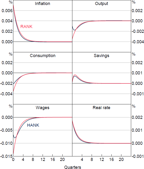
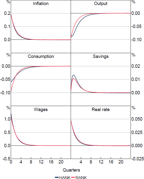
First, we examine a basic monetary policy shock to illustrate how heterogeneity in liquid asset savings impacts the response of the economy to a prototypical disturbance. In particular, we introduce an exogenous 50 basis point reduction in the nominal rate. The results are shown in Figure 1.
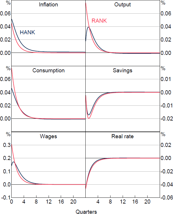
The response of inflation to the interest rate shock is largely consistent across models both with and without heterogeneous agents, displaying slight amplification with incomplete asset markets and a slower return to the steady-state rate. Correspondingly, the response of the real interest rate does not meaningfully differ as the central bank sets a similar nominal policy rate in both environments. Household savings adjust slightly less in the heterogeneous agent model.
On the real side of the economy, however, we see that real wages increase by less in the HANK version. As such, output rises by less with heterogeneous agents, with the initial output response only about a third of that with a representative agent. Notably, the initial consumption response with heterogeneous agents is only about two-thirds of that in RANK. The dampened real effects of a monetary policy shock in the HANK model contrast those found in much of the broader HANK and two-agent New Keynesian (TANK) literature.[3] Most such studies find that monetary policy shocks are amplified by heterogeneity in the HANK model. This is primarily due to a significant proportion of individuals whose assets are illiquid (or non-existent in the case of TANK) and cannot be used to smooth through the shock. This group's immediate consumption is primarily dictated by their current income, meaning they are more sensitive to changes in the various components of their income flows. In particular, Kaplan et al (2018) find that this income effect is very important. In contrast, we observe a large volume of liquid savings in the economy, which allows people to intertemporally smooth their consumption. This results in smaller deviations in consumption in response to shocks than from other variables. As a consequence, despite the sharp near-term decline in the stock of savings under the HANK model, the presence of ample savings and the ability to smooth consumption over time may somewhat mitigate the immediate impact of monetary policy shocks on consumption. This highlights the importance of including additional assets for empirical relevance of the model.
While the aggregate impulse responses show the overall effect of the shock on the heterogeneous agent economy, and convey the full extent of the transmission mechanism in the representative agent model, they are only a small piece of the story for transmission in the heterogeneous agent model. In particular, in HANK there is a non-trivial distribution of households over income and net worth states at each time t. Because these households have different levels of savings and income, their optimal responses to the shock differ. It is these optimal decisions that combine to give the aggregate results.
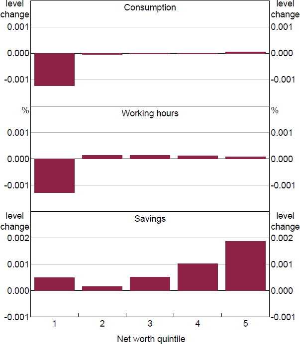
Figure 2 shows how decisions of agents change in response to the monetary easing shock, immediately after the shock, for each quintile of the net worth distribution. The quintiles are arranged on the horizontal axis, with the leftmost quintile being the least wealthy 20 per cent of households, the next over being the next least wealthy 20 per cent, and so on. The heights of the bars represent the average across the quintile of the change in optimal consumption, working hours, and savings from their steady-state values.
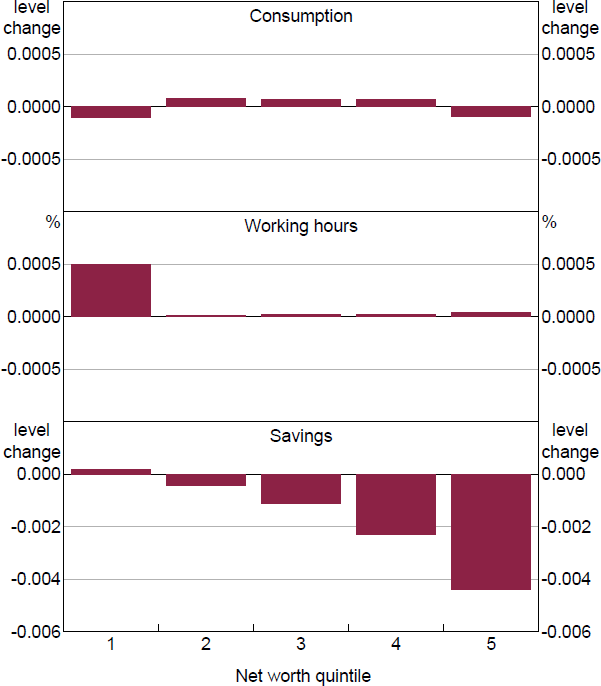
We see from the plot that high-wealth individuals, having received a large hit to their investment income, reduce bond holdings to partially smooth consumption. Despite their ability to do so, however, consumption smoothing is not complete and these agents do reduce consumption in response to the loss of income. Meanwhile, low-income individuals take advantage of the increase to real wages to work more and build up some liquid savings. For the middle of the distribution, we have the usual dynamics we would expect to see in RANK, wherein lower interest rates motivate intertemporal substitution: households sell asset holdings to increase current consumption.
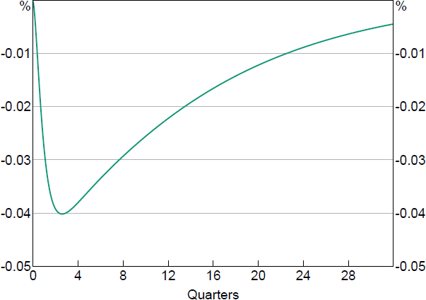
The HANK model also allows us to analyse the dynamics of wealth inequality in response to shocks, for example, by examining the response of the wealth Gini coefficient to the shock.[4] In this context the Gini coefficient summarises the overall degree of net worth inequality in the economy. A Gini coefficient of zero would imply total equality, while a Gini coefficient of one would suggest that all the wealth in the economy is concentrated at the top end of the distribution. Moreover, if wealth rose proportionally across all individuals, the Gini coefficient would not change – even though those with larger amounts of wealth would have a greater absolute amount of wealth. In this way, this measure is focused on the relative inequality in wealth between people – not the absolute magnitude of wealth.
Monetary policy easing in this environment leads to a reduction in the wealth Gini coefficient by 0.04 per cent from its steady-state level, reaching its trough in approximately the fourth quarter (Figure 3). This means that outcomes are more equal. Note that the fall in the Gini coefficient observed here is consistent with the response of household individual behaviour described above. Namely, low-wealth households increase their savings and high-wealth households decrease their savings in response to the shock, bringing the distribution closer together. Moreover, the adjustment to wealth inequality is persistent, taking a long time to return to the steady-state level.
While empirical studies on the impact of monetary policy on wealth inequality are sparse, these results can be compared to the body of empirical literature on the impacts of monetary policy on income inequality, insofar as these two dimensions of inequality are likely to be linked. For example, Aye, Clance and Gupta (2019) use quarterly time series data for the United States, finding that contractionary monetary and fiscal policies increase inequality across a broad range of metrics including income. Similarly, Coibon et al (2017) examine consumption and income inequality as measured in the Consumer Expenditure Surveys in the United States, also finding that contractionary monetary shocks increase inequality. Furceri, Loungani and Zdzienicka (2018) use income inequality data from the Standardized World Income Inequality Database (SWIID) to examine the effect of monetary policy on a panel of 32 advanced and emerging market economies, finding that contractionary policy increases inequality on average. Likewise, Mumtaz and Theophilopoulou (2017) find that contractionary policy exacerbates earnings, income, and consumption inequality in the United Kingdom. One contrasting result is that of Villarreal (2014), who found that contractionary monetary shocks are correlated with declines in income inequality in Mexico.
6.2 Supply-side shocks
Next, we examine the responses of the model economies to two shocks on the supply side.
Labour supply shock: The shock to labour supply we consider here is disturbance to a parameter in the household optimisation problem. In particular, this enters directly into Equation (9). When the functional form for the utility function in Equation (2) is substituted into this equation and the time dependence of preference parameters made explicit, it reads
The shock we now consider is that to .
Consider an increase to , which increases the weight on disutility from working. This direct impact of the shock is to increase the left-hand side of Equation (26), reflecting an increase in the marginal disutility from work. Equality can then be restored by a pair of endogenous responses by the household. For one, the household could reduce its labour hours until marginal disutility from working once again balanced with marginal utility from consumption. Alternatively, the household could reduce its consumption to restore this balance. Note the sense in which these decisions would be complementary through the household budget constraint: a reduction in labour hours would reduce wage income, which in turn could lead to lower consumption.
A third possibility not dependent on the household changing its own behaviour would be for wages to increase. This could happen due to firms in the economy discovering that all of their employees are reducing hours worked due to a common loss in utility from these hours, and using wages to try to entice these hours up to meet demand. In the model, it is likely that all three effects will occur simultaneously. Moreover, there are additional, general equilibrium effects which take place as households on average adjust their consumption and hours, with flow on effects to prices, interest rates, and savings.
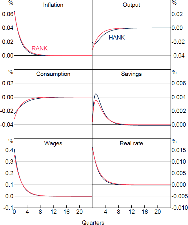
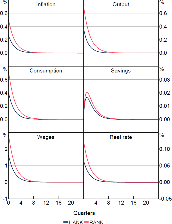
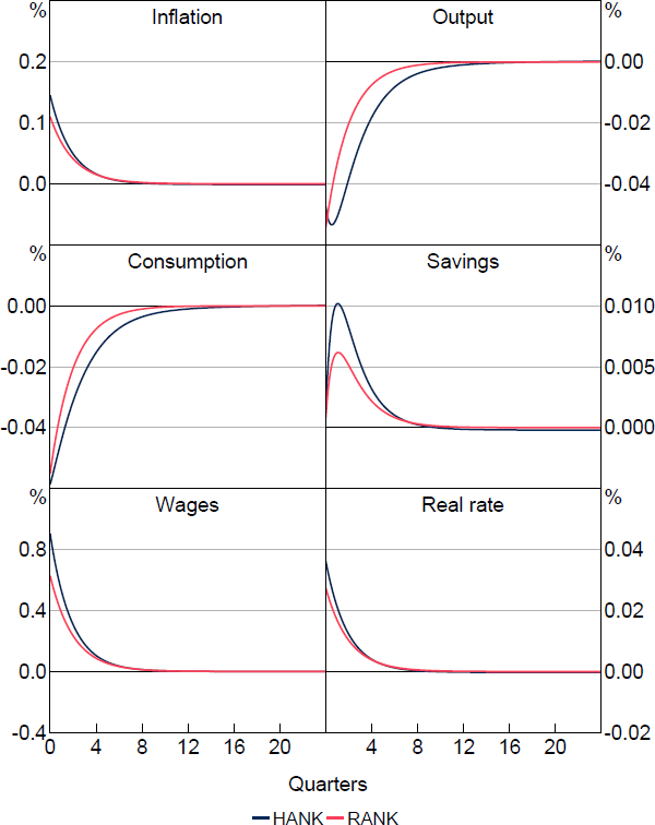
The aggregate responses to the labour disutility shock are shown in Figure 4. We observe that in both HANK and RANK, all three of the above responses do indeed occur: consumption drops, working hours drop, and wages increase. As with a monetary policy shock, the effect on consumption and output is less in the HANK model relative to the RANK model. In particular, the initial impact of the shock on output in the heterogeneous agent model is only about 71 per cent of that in the representative agent model, while for consumption it is only 81 per cent. Despite this, the responses in HANK are more persistent than in RANK, and after about two quarters the former dominate. In contrast, prices in the economy react almost identically in both models, while savings accumulate more in HANK.
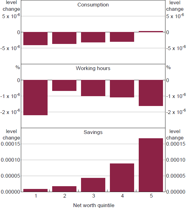
As with a monetary policy shock, we can further examine the transmission mechanism in the heterogeneous agent model by examining how household behaviour changes across the distribution of wealth, shown in Figure 5. Here we see that the drop in hours is actually entirely due to a strong response by only the poorest agents, while the remainder of the distribution actually increase hours worked. This positive response of working hours ultimately reflects a higher real wage, enticing agents to supply additional labour in spite of the change in their preferences.
Consumption also responds most strongly for the bottom quintile in response to the rise in disutility from working. This is because low-income households work the most hours. So the rise in disutility has the biggest effect on them, resulting in a big fall in consumption.
Finally, all agents in the model increase their savings, with wealthy agents increasing by the most, and declining down to the second quintile. The poorest agents, meanwhile, increase savings by about as much as the third quintile. This suggests that, despite working becoming less attractive, overall household income flows remain robust following the shock, once again due to the adjustment of real wages and increased hours worked. Indeed, the inflation generated by the shock causes a response by the central bank through the Taylor rule, and real interest rates rise. For net savers, this produces additional income from savings, and moreover as noted above these households actually increase working hours. For poor households, an increase in savings requires the sharp decline in consumption noted above, although the rise in wages would somewhat offset the cut in hours worked for these households.
Mark-up shock: We conclude by examining a supply side shock which directly impacts the firms' optimisation condition, given by Equation (19). We can rewrite this equation as
where we have now included a time subscript on the parameter , to reflect the fact that it is now subject to an exogenous disturbance. In particular, we consider a shock that decreases , with the interpretation that firms have more market power, given by Equation (11).
This shock has two direct impacts on the equilibrium condition above. First, it decreases the term in parentheses on the right. Since this term appears with a negative sign, this increases the full term in parentheses, and hence increases the right-hand side. Intuitively, the reciprocal of this term gives the firms' desired price mark-up above their marginal costs absent price rigidities, reflecting the fact that less substitutability increases individual firm market power. The second effect the shock has is to decrease the factor , indicating a flattening of the Phillips curve as the state of the real economy becomes less of a factor in firm pricing decisions.
Given our parameter values and the resultant steady-state wage rate, the net effect of the shock is to increase the right side of the above equilibrium condition, absent any adjustment of other variables. As in the case of labour supply, there are a number of potential mechanisms by which the economy can balance this condition. For example, inflation could increase on the left-hand side, as firms exercise their newly established market power to increase margins. However, this has the effect of increasing expectations about future inflation on the right-hand side. Similarly, the expected growth rate of output could decrease on the right-hand side. Lastly, wages could adjust downwards.
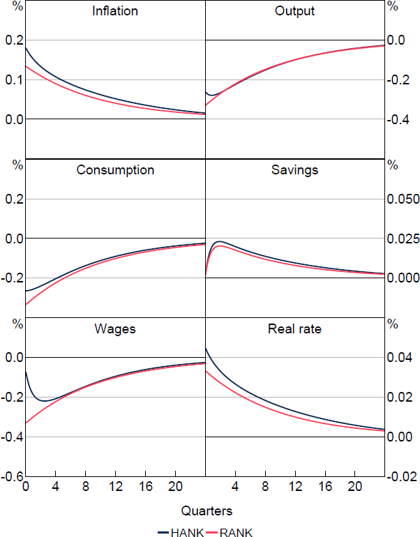
Figure 6 displays the aggregate impacts of the shock, once again demonstrating that all three effects take place. Inflation rises by about the same amount in the model with or without heterogeneous agents once again, but the disruptions to output and consumption are much less significant with heterogeneity. In particular, the response of output on impact in the HANK model is only 0.27 times that in RANK, although it is a bit more persistent in later periods. Likewise, the consumption response with heterogeneous agents is only 0.59 times that without. In contrast to the case of a labour supply shock, wages decline in both models, although yet again the effect is dampened in the heterogeneous agent model by a factor of 0.48.
Turning to the transmission mechanism in the heterogeneous agent model, Figure 7 shows how agents across the quintiles of the distribution of wealth react on impact to a substitutability between goods shock. The increase in market power allows firms to increase prices and to maintain profits while supplying less output. This leads to a jump in inflation and a decline in demand for labour, lowering wages. For households, this results in a decline in working hours across the entire distribution.
The central bank responds to inflation by increasing interest rates, motivating households to increase savings, once again across the entire distribution. However, the loss in labour income, combined with the increase in prices, results in savings rates varying significantly between wealth brackets. Moreover, the first four quintiles of the distribution cut back on consumption. On the other hand, the wealthiest households, whose increase in interest income more than offsets the decline in wages and the increase in consumer prices, are able to increase their consumption as well as disproportionately increase their savings.
These results suggest that, while household heterogeneity may have relatively strong implications for the transmission of both supply and demand shocks that directly impact the household optimisation problem, it may be less critical for understanding supply shocks that impact the firm side initially.
In particular, while inspection of the wealth Gini coefficent indicates that inequality goes up in response to both of the supply shocks we have considered, the maximum increase is two orders of magnitude smaller for the mark-up shock than for either the monetary policy or labour disutility shock, despite the fact that both supply shocks are calibrated to have the same degree of persistence and magnitude. Nonetheless, the dampening of the overall impact once again underscores the importance of capturing liquidity and other potential constraints. Finally, while it may not be surprising that household heterogeneity is more important for shocks which impact households, there is also diversity among firms in the economy, and this type of heterogeneity may be more critical for the transmission of these types of shocks.
7. Conclusion
In this paper, we've begun to investigate incorporating heterogeneity into a macroeconomic model of the Australian economy. Specifically, we've explored how a model with uninsurable individual productivity shocks will result in households in the model having different optimal decisions, resulting in a distribution of these households over wealth and income. We've then examined how these differences impact how aggregate economic shocks transmit through the economy.
This work comes at a time of heightened interest both in how heterogeneity impacts shock transmission to the economy, and how they impact distributional outcomes. In terms of shock transmission, differing agent behaviour in one part of the distribution could offset that in another, while agents at constraints could amplify the effects. In terms of distributional outcomes, some agents may be made worse off by a given shock depending on their history of asset accumulation whereas others might be made better off.
The specific exercise in this paper was to construct a HANK model – featuring heterogeneous agents differing in income and wealth, price rigidities and a role for monetary policy – calibrated to the income dynamics of the Australian economy. We found that in such a model, real effects of monetary policy shocks, labour supply shocks, and mark-up shocks tend to be dampened due to high household insurance through a large stock of liquid assets. We also found that these shocks resulted in a variation of household reactions across the distribution, while the distributional impacts of mark-up shocks were relatively subdued.
Notably, the results with regards to a demand shock in this paper are at odds with the wider literature, which typically finds amplification of shocks with heterogeneous agents. While this work is an important first step towards understanding how the range of income and wealth outcomes in the Australian economy can impact the transmission of economic shocks, it also highlights the importance of further work to understand how incorporating a broader range of assets into the model would affect this transmission. These issues, among others, highlight the potential value of further structural modelling of the Australian economy.
Appendix A: Shock Responses Not Discussed in the Main Text
References
Acharya S and K Dogra (2018), ‘Understanding HANK: Insights from a PRANK’, Paper presented at the 2018 Annual Meeting of the Society for Economic Dynamics, Mexico City, 28–30 June.
Ahn S, G Kaplan, B Moll, T Winberry and C Wolf (2017), ‘When Inequality Matters for Macro and Macro Matters for Inequality’, in M Eichenbaum and JA Parker (eds), NBER Macroeconomics Annual, 32, University of Chicago Press, Chicago, pp 1–75.
Aiyagari SR (1994), ‘Uninsured Idiosyncratic Risk and Aggregate Saving’, The Quarterly Journal of Economics, 109(3), pp 659–684.
Auclert A, M Rognlie, M Souchier and L Straub (2021), ‘Exchange Rates and Monetary Policy with Heterogeneous Agents: Sizing up the Real Income Channel’, NBER Working Paper No 28872, rev August 2024.
Auclert A, M Rognlie and L Straub (2020), ‘Micro Jumps, Macro Humps: Monetary Policy and Business Cycles in an Estimated HANK Model’, NBER Working Paper No 26647.
Aye GC, MW Clance and R Gupta (2019), ‘The Effectiveness of Monetary and Fiscal Policy Shocks on U.S. Inequality: The Role of Uncertainty’, Quality & Quantity, 53(1), pp 283–295.
Barro RJ and RG King (1984), ‘Time-separable Preferences and Intertemporal-substitution Models of Business Cycles’, The Quarterly Journal of Economics, 99(4), pp 817–839.
Bewley T (1977), ‘The Permanent Income Hypothesis: A Theoretical Formulation’, Journal of Economic Theory, 16(2), pp 252–292.
Cantore C, F Ferroni, H Mumtaz and A Theophilopoulou (2023), ‘A Tail of Labor Supply and a Tale of Monetary Policy’, Centre for Macroeconomics Discussion Paper No CFM-DP2023-08.
Chipeniuk K and G Nolan (2022), ‘Monetary Policy Easing and the Distribution of Wealth in New Zealand’, Reserve Bank of New Zealand Analytical Note AN2022/01.
Christiano LJ, M Eichenbaum and CL Evans (1999), ‘Monetary Policy Shocks: What Have We Learned and to What End?’, in JB Taylor and M Woodford (eds), Handbook of Macroeconomics: Volume 1A, Handbooks in Economics 15, Elsevier Science, Amsterdam, pp 65–148.
Coibion O, Y Gorodnichenko, L Kueng and J Silvia (2017), ‘Innocent Bystanders? Monetary Policy and Inequality’, Journal of Monetary Economics, 88, pp 70–89.
Faccini R, S Lee, R Luetticke, M Ravn and T Rankin (2024), ‘Financial Frictions: Micro vs. Macro Volatility’, Danmarks Nationalbank Working Paper No 200.
Fernández-Villaverde J (2010), ‘The Econometrics of DSGE Models’, SERIEs: Journal of the Spanish Economic Association, 1(1–2), pp 3–49.
Furceri D, P Loungani and A Zdzienicka (2018), ‘The Effects of Monetary Policy Shocks on Inequality’, Journal of International Money and Finance, 85, pp 168–186.
Guo F, IK-M Yan, T Chen and C-T Hu (2023), ‘Fiscal Multipliers, Monetary Efficacy, and Hand-to-mouth Households’, Journal of International Money and Finance, 130, Article 102743.
Guvenen F, F Karahan, S Ozkan and J Song (2019), ‘What Do Data on Millions of U.S. Workers Reveal about Life-cycle Earnings Dynamics?’, Federal Reserve Bank of New York Staff Report No 710.
Heathcote J (2005), ‘Fiscal Policy with Heterogeneous Agents and Incomplete Markets’, The Review of Economic Studies, 72(1), pp 161–188.
Kaplan G, B Moll and GL Violante (2018), ‘Monetary Policy According to HANK’, The American Economic Review, 108(3), pp 697–743.
Kaplan G and GL Violante (2018), ‘Microeconomic Heterogeneity and Macroeconomic Shocks’, Journal of Economics Perspectives, 32(3), pp 167–194.
Krueger D, K Mitman and F Perri (2016), ‘Macroeconomics and Household Heterogeneity’, in JB Taylor and H Uhlig (eds), Handbook of Macroeconomics: Volume 2A, Handbooks in Economics, Elsevier, Amsterdam, pp 843–921.
Krusell P and AA Smith, Jr (1998), ‘Income and Wealth Heterogeneity in the Macroeconomy’, Journal of Political Economy, 106(5), pp 867–896.
Leong J (2021), ‘An Overview of the Distributional Effects of Monetary Policy’, Reserve Bank of New Zealand Analytical Note No AN2021/5.
Mumtaz H and A Theophilopoulou (2017), ‘The Impact of Monetary Policy on Inequality in the UK. An Empirical Analysis’, European Economic Review, 98, pp 410–423.
Reiter M (2009), ‘Solving Heterogeneous-agent Models by Projection and Perturbation’, Journal of Economic Dynamics & Control, 33(3), pp 649–665.
Villarreal FG (2014), ‘Monetary Policy and Inequality in Mexico’, Munich Personal RePEc Archive MPRA Paper No 57074.
Copyright and Disclaimer Notice
BLADE Disclaimer
The following Disclaimer Notice refers to data and graphs sourced from the Australian Bureau of Statistics' BLADE (Business Longitudinal Analysis Data Environment) database.
The results of these studies are based, in part, on data supplied to the ABS under the Taxation Administration Act 1953, A New Tax System (Australian Business Number) Act 1999, Australian Border Force Act 2015, Social Security (Administration) Act 1999, A New Tax System (Family Assistance) (Administration) Act 1999, Paid Parental Leave Act 2010 and/or the Student Assistance Act 1973. Such data may only be used for the purpose of administering the Census and Statistics Act 1905 or performance of functions of the ABS as set out in section 6 of the Australian Bureau of Statistics Act 1975. No individual information collected under the Census and Statistics Act 1905 is provided back to custodians for administrative or regulatory purposes. Any discussion of data limitations or weaknesses is in the context of using the data for statistical purposes and is not related to the ability of the data to support the Australian Taxation Office, Australian Business Register, Department of Social Services and/or Department of Home Affairs' core operational requirements.
Legislative requirements to ensure privacy and secrecy of these data have been followed. For access to MADIP and/or BLADE data under Section 16A of the ABS Act 1975 or enabled by section 15 of the Census and Statistics (Information Release and Access) Determination 2018, source data are de-identified and so data about specific individuals has not been viewed in conducting this analysis. In accordance with the Census and Statistics Act 1905, results have been treated where necessary to ensure that they are not likely to enable identification of a particular person or organisation.
Acknowledgements
The authors would like to acknowledge contributions by Sarah Hunter, Jonathan Hambur, Ekaterina Shabalina, Dennis Wesselbaum, the RBA's Economic Research Department staff and participants at the 2022 VAMS workshop. The views expressed in this paper are those of the authors and should not be attributed to the Reserve Bank of Australia, the Reserve Bank of New Zealand or the e61 Institute. Any errors are the sole responsibility of the authors.
Footnotes
In particular, Kaplan et al (2018) use seven moments, namely the variances of log earnings, their one-year change, and their five-year change, the kurtosis of their one-year and five-year changes, as well as the fraction for which the one-year change was less than 10, 20, and 50 per cent. [1]
Results given for the United States use the productivity process estimated in Kaplan et al (2018), while those for New Zealand are taken from Chipeniuk and Nolan (2022). [2]
It is worth noting that we find larger real effects in HANK than in RANK under alternative parameter specifications. For example, setting the Frisch elasticity to be 0.85 as in Fernández-Villaverde (2010) results in a consumption response that is about 33 per cent larger in HANK. This choice of calibration also results in supply responses that are much more persistent in HANK than in RANK. [3]
The decline in the wealth Gini coefficient occurs in the absence of capital gains, and is driven by the loss of interest income at the top end of the distribution. Moreover, distributional impacts are likely to run in the opposite direction for an interest rate increase, suggesting that the impacts may be negligible over a full cycle. [4]