RDP 2021-02: Star Wars at Central Banks 5. Our Findings Do Not Call for Changes in Research Practices
February 2021
- Download the Paper 1,553KB
5.1 The p-curve produces no evidence of bias
Using the p-curve method, we do not find any statistical evidence of researcher bias in our central bank sample. In fact, the p-curve shows an obvious downward slope (Figure 4). We get the same qualitative results when applying the p-curve to the top journals dataset, even though Brodeur et al (2016) do find evidence of researcher bias when applying the z-curve to that dataset. While our finding is consistent with the p-curve's high propensity to produce false negatives, it is not necessarily an example of one.
Our pre-analysis plan also specifies p-curve assessments of several subgroups, and includes several methodological robustness checks. The results are all the same: we find no evidence of researcher bias, since the p-curves all slope downward. We have little more of value to say about those results, so we leave the details to our online appendix.
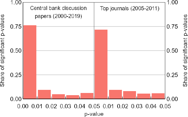
Note: The observed p-curves from both samples are clearly downward sloping, a result that does not suggest researcher bias.
Sources: Authors' calculations; Brodeur et al (2016); Federal Reserve Bank of Minneapolis; Reserve Bank of Australia; Reserve Bank of New Zealand
5.2 The z-curve results show just as much bias at central banks as at top journals
For central banks, the observed distribution of z-scores for the main results (not the controls), and without any of our sample changes, is unimodal (Figure 1). For top journals, the equivalent distribution is bimodal. The difference matters because it is the bimodal shape that motivates the z-curve decomposition conducted by Brodeur et al (2016). The difference is thus evidence suggestive of differences in researcher bias.
The formal results of the z-curve in Table 2, however, show roughly as much researcher bias at central banks as in top journals. The number 2.3 in the first column of data technically reads as ‘assuming that the bias-free form of P[z] is the Cauchy distribution with 1.5 degrees of freedom, and P[disseminated|z] is well estimated non-parametrically, there is an unexplained excess of just-significant results that amounts to 2.3 per cent of all results’. The excess is what Brodeur et al (2016) attribute to researcher bias, so higher numbers are worse. The result is meant to be conservative because the z-curve method tries to explain as much of P[z|disseminated] as possible with dissemination bias. The empty cells in Table 2 correspond to what turned out to be poor candidates for bias-free P[z], as judged by Step 2 of the z-curve method.
| Assumed P[z] | Central banks | Top journals | |||
|---|---|---|---|---|---|
| Non-parametric estimate of P[disseminated|z] | Parametric estimate of P[disseminated|z] | Non-parametric estimate of P[disseminated|z] | Parametric estimate of P[disseminated|z] | ||
| Standard | |||||
| Student-t(1) | 1.7 | 2.5 | |||
| Cauchy(0.5) | 1.1 | 1.6 | |||
| Cauchy(1.5) | 2.3 | 2.9 | |||
| Empirical | |||||
| WDI | 2.2 | 2.7 | 2.7 | 3.0 | |
| VHLSS | 1.8 | 2.0 | 2.0 | 2.0 | |
| QOG | 1.2 | 1.7 | 1.4 | 2.0 | |
| PSID | 1.4 | 2.3 | |||
|
Notes: The number 2.3 in the first column of data reads as ‘there is an unexplained excess of just-significant results that amounts to 2.3 per cent of all results’. The z-curve method attributes this excess to researcher bias. We drop one-sided tests from the Brodeur et al (2016) sample, but the effect is negligible. The empty cells correspond to what turned out to be poor candidates for bias-free P[z], as per our pre-analysis plan. Sources: Authors' calculations; Brodeur et al (2016); Federal Reserve Bank of Minneapolis; Reserve Bank of Australia; Reserve Bank of New Zealand |
|||||
Brodeur et al (2016) support their main results with many figures, including several that (i) justify their choices for bias-free forms of P[z], (ii) show their estimated functional forms for P[disseminated|z], and (iii) show the cumulative portions of estimated P[z|disseminated] that cannot be explained with P[z] and P[disseminated|z]. These last ones plot the supposed influence of researcher bias. In our work, the most interesting finding from the equivalent sets of figures is that we generate all of the results in Table 2 using sensible functional forms for P[disseminated|z]. For example, the functional forms that we estimate non-parametrically all reach their peak (or almost reach it) at the |z| = 1.96 threshold and are little changed over higher values of absolute z. This is consistent with the assumption in both methods that P[disseminated|z] is not a source of distortion for high absolute z. To simplify and shorten our paper, we leave these extra figures to our online appendix.
5.3 Our extensions cast doubt on the z-curve method
Within our central bank sample, hypothesis tests disclosed as coming from data-driven model selection or reverse causal research yield distributions of test statistics that look quite different from the rest (Figure 5). None of the distributions show obvious anomalies, but had central banks done more data-driven model selection or reverse causal research, the combined distribution in the left panel of Figure 1 could plausibly have been bimodal as well. Likewise, the observed bimodal shape for the top journals might occur because they have a high concentration of data-driven model selection and reverse causal research; we just do not have the necessary data to tell. Unsurprisingly, these types of test statistics also exaggerate our formal z-curve results; if we apply the z-curve method to the central bank sample that excludes data-driven model selection and reverse causal research, our bias estimates fall by about a third (Table 3).
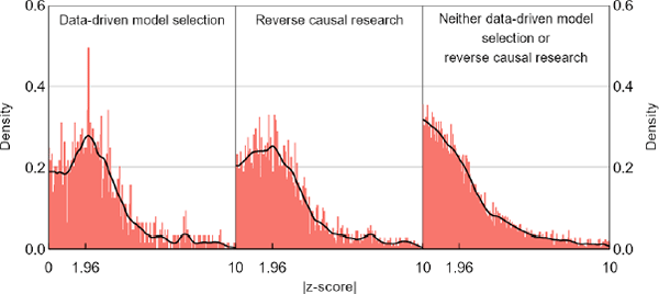
Notes: Data-driven model selection and reverse causal research are overlapping categories. None of the distributions show obvious anomalies, but if they were blended with different weights, they could plausibly produce a bimodal aggregate.
Sources: Sources: Authors' calculations; Federal Reserve Bank of Minneapolis; Reserve Bank of Australia; Reserve Bank of New Zealand
| Assumed P[z] | Main sample excluding data-driven model selection and reverse causal research | Placebo sample on control variable parameters | |||
|---|---|---|---|---|---|
| Non-parametric estimate of P[disseminated|z] | Parametric estimate of P[disseminated|z] | Non-parametric estimate of P[disseminated|z] | Parametric estimate of P[disseminated|z] | ||
| Standard | |||||
| Cauchy(0.5) | 1.6 | 2.2 | 2.1 | 1.7 | |
| Cauchy(1.5) | 3.4 | 2.8 | 2.4 | 2.6 | |
| Empirical | |||||
| WDI | 1.5 | 1.9 | 2.1 | 1.7 | |
| VHLSS | 1.2 | 1.4 | 2.2 | 1.5 | |
| QOG | 0.7 | 1.1 | 2.0 | 0.8 | |
|
Notes: The number 1.6 in the first column of data reads as ‘there is an unexplained excess of just-significant results that amounts to 1.6 per cent of all results’. The z-curve method attributes this excess to researcher bias. The placebo sample is at a size that Brodeur et al (2016) say is too small to reliably use the z-curve method. Acknowledging that, it produces just as much measured researcher bias as the cleansed main sample. We add results that correspond to a Cauchy distribution with 0.5 degrees of freedom for P[z] because the observed test statistics here show thicker tails than for the main sample. This is especially true of the control variables distribution. Sources: Authors' calculations; Brodeur et al (2016); Federal Reserve Bank of Minneapolis; Reserve Bank of Australia; Reserve Bank of New Zealand |
|||||
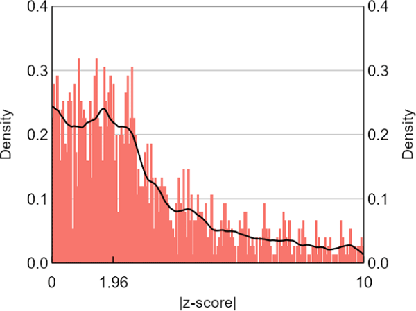
Our placebo exercise also casts doubt on the z-curve method. Our sample of controls is around sizes that Brodeur et al (2016) regard as too small to reliably use the z-curve method, so the controls distribution of test statistics is noisier than the others (Figure 6) and our placebo test is only partial. In any event, our formal z-curve results for the controls sample show just as much researcher bias as for the main sample, after we exclude from it results produced by data-driven model selection or reverse causal research (Table 3). Ideally, the tests would have shown no measured researcher bias, because there is no incentive to produce statistically significant results for control variables. It is thus difficult to attribute the formal z-curve results for our central bank sample to researcher bias.
Sources: Authors' calculations; Federal Reserve Bank of Minneapolis; Reserve Bank of Australia; Reserve Bank of New Zealand
5.4 Differences in dissemination bias might be important here
What then might explain the differences between our sample distributions of z-scores for the central banks and top journals? The differences must come from P[disseminated|z], unbiased P[z], researcher bias, sampling error, or some combination of these factors, but we have insufficient evidence to isolate which. There is a lot of room for speculation here and, judging by our conversations with others on this topic, a strong appetite for such speculation as well. Here, we restrict our comments to the few we can support with data.
As per the stylised scenario in Figure 2, one possible explanation for the bimodal shape of the top journals distribution could be a steep increase in P[disseminated|z] near significant values of z. Likewise, the absence of bimodality at the central banks might reflect a shallower increase in P[disseminated|z].[9] The z-curve method does produce estimates of P[disseminated|z] – as part of Step 3 – and they are consistent with this story (Figure 7). However, the problems we have identified with the z-curve method would affect these estimates as well.
![Figure 7: Comparisons of Estimated P[disseminated|z]](images/figure-7.gif)
Notes: The panels show estimated functions for P[disseminated|z] for different versions of P[z], but always using the non-parametric estimation method outlined in Brodeur et al (2016). The probabilities have also been indexed to 100 at |z| = 1.96 to facilitate comparison. The estimated functions are steeper in the almost-significant zone for top journals than they are for central banks.
Sources: Authors' calculations; Brodeur et al (2016); Federal Reserve Bank of Minneapolis; Reserve Bank of Australia; Reserve Bank of New Zealand
Whatever the sources of the distributional differences, they are unlikely to stem from central banks focusing more on macroeconomic research, at least as broadly defined. Brodeur et al (2016) show a sample distribution that uses only macroeconomic papers, and it too is bimodal. In fact, bimodality features in just about all of the subsamples they present.
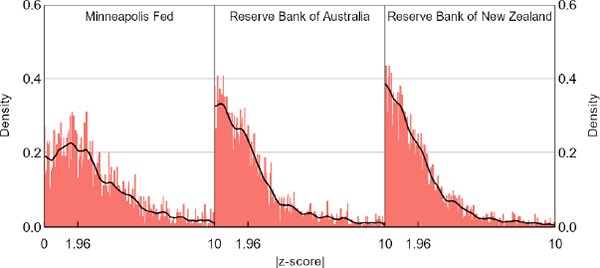
We also doubt that the sources of the distributional differences could apply equally to the 3 central banks we analyse. Noting that our sample sizes for each of them are getting small, the data for the Minneapolis Fed look like they come from a population with more mass in high absolute z (Figure 8). This right-shift is consistent with our subjective view of differences in publication incentives, but since our summary statistics show that the Minneapolis Fed stands out on several other dimensions as well, we are reluctant to push this point further. Moreover, restricting our central bank sample to papers that were subsequently published in journals does not produce a distribution noteworthy for its right-shift (Figure 9). This result surprised us. Further work could investigate whether the journal versions of these same papers produce noticeable distributional shifts. O'Boyle, Banks and Gonzalez-Mulé (2017) do a similar exercise in the field of management, finding that the ratio of supported to unsupported hypotheses was over twice as high in journal versions of dissertations than in the pre-publication versions.
Sources: Authors' calculations; Federal Reserve Bank of Minneapolis; Reserve Bank of Australia; Reserve Bank of New Zealand
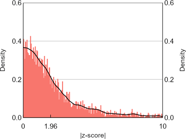
Note: Restricting the central bank sample to papers that were subsequently published in journals does not produce a distribution of test statistics that is noteworthy for its right-shift.
Sources: Authors' calculations; Federal Reserve Bank of Minneapolis; Reserve Bank of Australia; Reserve Bank of New Zealand
Footnote
Dissemination is defined by the dataset being used. In the top journals dataset, dissemination refers to publication in a top journal, while in the central banks dataset, dissemination refers to inclusion in a discussion paper that has been released on a central bank's website. [9]