Research Discussion Paper – RDP 2020-07 How Many Jobs Did JobKeeper Keep?
1. Introduction
The COVID-19 outbreak in Australia in early 2020 led to a sharp fall in economic activity. In response, the Australian Government announced a series of measures to support incomes and employment. The largest single measure was the $101.3 billion wage subsidy scheme called the ‘JobKeeper Payment’. As its name implies, a key objective of the JobKeeper Payment was to preserve the connections between employers and their employees during the crisis, and to support business and job survival. It did this by giving employers a wage subsidy for eligible employees in order to help them retain those employees and reduce the associated wage costs. Another objective of JobKeeper was to provide income support. In the initial six-month stage of the program (30 March 2020 to 27 September 2020), which is the focus of our paper, the subsidy was paid as a flat $1,500 per fortnight for each eligible employee.
The JobKeeper Payment is one of the largest labour market interventions in Australia's history (Australian Government 2020b). In its first six months, it supported around 3.5 million workers in more than 900,000 businesses, and undoubtedly played a crucial role in cushioning the decline in employment and incomes over the first half of 2020.[1] The Treasury's (2020b) three-month review of the program used descriptive evidence to make the assessment that JobKeeper has had a material effect. To date, however, no study has estimated the causal effect of the subsidy on employment using an approach that accounts for the differences between workers who received JobKeeper and those who did not. For this reason, the effect of JobKeeper on employment remains an open question. Our paper helps to fill this gap in the evidence base.
Specifically, we seek to answer the following question: what effect did JobKeeper have on employment during the first four months of the program? In doing so, we provide the first quantitative estimates of the causal effect of JobKeeper on employment, which build on the descriptive evidence discussed by Treasury (2020b). Our goal is to estimate the counterfactual – that is, how much employment would have fallen in the absence of JobKeeper. We find that one in every five employees who received JobKeeper would have exited employment had it not been for the wage subsidy. Scaling our estimates up to the aggregate level suggests that JobKeeper reduced overall employment losses by at least 700,000 during its first four months (Figure 1). While our error bands are wide and our analysis has a number of important caveats, our findings are close to Treasury's ex post and ex ante estimates of the number of jobs that the program ‘saved’.
To identify the causal effect of JobKeeper on employment, we make use of a strict threshold in the eligibility criteria for the program. We compare the employment outcomes of casual employees who had a little less than 12 months of tenure with their employer in early March (who narrowly missed out on being eligible for JobKeeper) to that of casuals with a little more than 12 months of tenure (who were potentially eligible). Because our approach focuses on casual employees in a narrow range of tenure, these two groups should be similar in terms of their observable and unobservable characteristics. As such, any differences between these groups that emerged after the introduction of JobKeeper can be attributed to the effects of the program rather than to other factors, such as the uneven effect of COVID-19 across industries. To implement this approach, we use individual-level data from the Labour Force Survey (LFS) and a difference-in-differences strategy.
Notes:
(a) Shaded area represents 95 per cent confidence intervals
(b) Based on Treasury estimates of effect of fiscal measures on employment
Sources: ABS; Australian Government (2020c, p 38); Authors' calculations
Our findings have implications for policy. First, a better understanding of the effects of JobKeeper on employment can provide additional guidance to policymakers on the benefits of extending (or costs of withdrawing) the scheme. While we do not perform a cost-benefit analysis, our results would be an important consideration in such an analysis. Second, our results will be useful for forecasters grappling with the question of whether the withdrawal of existing support measures in late 2020 and early 2021 will have implications for labour market outcomes and economic growth. For example, it may be reasonable to assume that the number of jobs saved by the introduction of JobKeeper provides an upper bound on the number of jobs that will be lost once the program ends. In saying that, any such employment losses could be offset by an underlying recovery in economic activity or further policy stimulus. It is reasonable to think that the effects of JobKeeper on employment will vary with the state of the labour market, and could plausibly be much lower by the time the scheme ends. Finally, as Treasury (2020b, p 39) have noted, a better understanding of the effects of JobKeeper can aid policymakers in the event of future economic shocks.
Throughout this paper we pay close attention to the assumptions that underpin our results. There are two that are worth emphasising upfront, because we were not able to test them in a rigorous way. The first of these key assumptions is that JobKeeper did not have spillover effects on workers who did not receive it, either at a firm level (for example, through its general support of firm profitability) or at an aggregate level via general equilibrium effects (for example, through its effect of supporting the overall strength of the economy). If this assumption does not hold, we may have either overstated or understated the effects of JobKeeper on employment depending on the nature of the spillover. The second key assumption is that the effects we estimate for casuals with limited job tenure can generalise to other JobKeeper recipients. That is, we assume that JobKeeper had similar effects on employment outcomes for casual employees as for permanent ones, notwithstanding that these employment relationships differ in a range of ways, as do the characteristics of the firms and workers who use them.
It is important to note that our analysis is entirely retrospective. Our focus is on how JobKeeper supported employment in the first few months of the program. We do not consider the effects of JobKeeper from August 2020 onwards. Notably, the changes in payment rates and eligibility that occurred from end September mean that our estimates may not generalise beyond our period of analysis. Treasury (2020b, p 7) has noted that JobKeeper has a ‘number of features that create adverse incentives which may become more pronounced over time as the economy recovers’.
An important policy question is whether JobKeeper was effective in alleviating the longer-run effects of labour market scarring. We do not consider this question in our paper. Even once the data become available, analysing these longer-run effects will be a more complicated task given the broader range of competing forces at play. An important avenue for future research will be to study the longer-term benefits and costs of the program on employment, earnings and productivity.
Another aspect of JobKeeper that our study does not consider explicitly is the role the program played in supporting incomes of firms and workers, which was one of its main objectives. As noted above, our analysis is also silent on the various indirect channels through which JobKeeper may have affected economic outcomes and employment in the first few months of the program, such as via second-round effects on aggregate demand. By focusing on the direct employment effects alone, our analysis provides a partial, albeit important, evaluation of the scheme.
The remainder of this paper is structured as follows. Section 2 provides some background on the JobKeeper Payment. Section 3 briefly discusses the existing evidence on JobKeeper and previous work on wage subsidy schemes. The data and empirical strategy are described in Sections 4 and 5. Sections 6 and 7 present the results and robustness tests. Section 8 provides our assessment of the short-run effect of JobKeeper and Section 9 provides some concluding remarks.
2. The JobKeeper Payment
2.1 Background
The outbreak of COVID-19 infections, along with the measures used to contain the spread of the virus, led to a sharp contraction in economic activity in Australia from around mid March 2020. The Australian Government responded by announcing a series of economic support packages in mid-to-late March. The single largest measure was the JobKeeper program, which provided a wage subsidy for businesses significantly affected by COVID-19 to help them retain and continue to pay their staff.
JobKeeper was announced on 30 March 2020 (effective immediately), and was originally scheduled to run for six months until end September 2020. The program had three objectives:
- to support business and job survival
- to preserve the employment relationship between employers and their workforce
- to provide income support to business owners and their workforce.
Our paper focuses on the second of these objectives (and, to a lesser extent, the first). Our study does not consider how effectively the program achieved its third objective of providing income support.
Although the program was originally due to end in September 2020, in July the government announced an extension until March 2021, albeit with some modified eligibility criteria and downward adjustments to payment rates (‘JobKeeper 2.0’). There were some further modifications announced in August in response to the increased social distancing restrictions in Victoria (Morrison and Frydenberg 2020). We do not study the effects of these changes or JobKeeper 2.0 in our paper. Instead, the focus of our paper is on the first four months of the program. In the remainder of our paper, any references we make to ‘JobKeeper’ or the ‘JobKeeper Payment’ will be referring specifically to this initial phase unless indicated otherwise.
2.2 Design Features
Under JobKeeper, eligible businesses were given a wage subsidy of $1,500 per fortnight for each eligible employee in order to help them retain those employees and reduce wage costs.[2] More specifically, eligible businesses that made wage payments of at least $1,500 per fortnight to an eligible worker were reimbursed that $1,500 amount in full by the Australian Taxation Office (ATO).[3]
There are several aspects of this payment design that warrant further discussion. First, the subsidy was paid as a flat per-worker rate: the value of the subsidy was the same for all covered workers regardless of the number of hours they worked during the program or their earnings. This flat rate distinguishes the JobKeeper Payment from the wage subsidy schemes used in most other OECD countries, which pay covered employees a proportion of their pre-scheme earnings up to a cap (RBA 2020).[4]
Second, the $1,500 payment rate also acted as a wage floor. If an eligible employee had been earning less than $1,500 per fortnight prior to the COVID-19 crisis, their employer needed to increase their wage payment to the $1,500 floor under the program.[5] This meant that many part-time employees were entitled to higher payments under JobKeeper than they would ordinarily receive.
The JobKeeper payment could also be extended to employees who had been ‘stood down’ by their employers. In this case, the employee would receive $1,500 per fortnight from their employer (who in turn was reimbursed by the ATO), even if they worked zero hours during the pay period. In this situation, the JobKeeper Payment is more akin to a transfer than a wage subsidy because the employee is transferred the full value of the subsidy without any production occurring (Treasury 2020b). People paid through JobKeeper could work less hours, the same hours, or more hours, than usual.
The legislation that accompanied JobKeeper also included some temporary changes to the Fair Work Act 2009 to give employers more flexibility to modify their employees' working arrangements while covered by the program. For example, an employee who received JobKeeper could have their hours reduced (including to zero), or be redeployed, at their employer's discretion. These provisions could override the conditions in the employees' employment contract that may otherwise have inhibited such flexibility. These provisions only applied to employees receiving JobKeeper, although other employees may also have been exposed to similar flexibility provisions given the temporary variations to certain modern awards. Previous research suggests that workplace-level flexibility can influence the extent to which firms adjust labour input by varying average hours rather than headcount (e.g. Bishop, Gustafsson and Plumb 2016). For this reason, it is possible the temporary flexibility provisions that accompanied JobKeeper had an effect on employment over and above the effect of the subsidy itself. Our analysis does not distinguish between these separate channels of effect.
2.3 Eligibility
The JobKeeper Payment program was designed to provide targeted support to businesses and workers who were adversely affected by COVID-19. To receive JobKeeper a job had to satisfy two tests:
- Worker eligibility: the worker had to be an Australian resident who was employed on 1 March as a permanent, fixed-term or ‘long-term casual’ – the latter refers to a casual employed for at least 12 months; and
- Firm eligibility: the firm must have experienced (or expect to experience) a fall in revenue of 30 per cent or more (for firms with less than $1 billion annual turnover) or 50 per cent or more (for firms with more than $1 billion annual turnover).[6]
This meant that an employee could have been working at an eligible firm but have been ineligible for JobKeeper if they were, say, a short-term casual, or if they were initially hired after the 1 March cut-off date.
Once a firm was enrolled in the program, they remained enrolled until the end of September, irrespective of how their revenues evolved or whether their expectations subsequently improved.
The relevant date for assessing worker eligibility was 1 March 2020.[7] An employee needed to be on the firm's books on this date in order to qualify for JobKeeper. Employees who were dismissed by their employer after 1 March but then subsequently re-engaged were eligible for the program, provided they were on the books as of 1 March and also met the other criteria. Employees who first joined the firm after 1 March were not eligible at that firm, and those who were eligible at one firm could not take that eligibility status with them to another firm if they changed jobs during the program (i.e. the subsidy was tied to worker-firm matches, not workers themselves). Given the eligibility date was one month prior to the announcement date and the program was developed very quickly, there is unlikely to have been an ‘anticipation effect’ on employment prior to the program announcement.
Casual employees faced some additional eligibility requirements. The program rules stipulated that a casual employee needed to have been employed at the business for at least 12 months on a regular basis in order to qualify. That is, their employer had to show that the employee had been engaged on or before 1 March 2019 and was still engaged on 1 March 2020. This 12-month tenure rule did not apply to employees on permanent or fixed-term contracts. We make use of this 12-month tenure rule to estimate the causal effect of JobKeeper on employment.
To enrol in the scheme, a firm had to log into the ATO website, make a series of declarations and provide their bank details (ATO 2020b; Hamilton 2020). If an eligible firm chose not to enrol, their eligible employees would not receive the subsidy at that firm. In saying that, conditional on eligibility, firm enrolment in the program was very high.[8] Firms could not selectively nominate employees to include under the scheme; any participating firm had to ensure that all of their eligible employees were covered by the program (a ‘one in, all in’ rule).[9] In cases where a worker had eligible jobs at more than one firm, only one firm was eligible to receive the JobKeeper payment on behalf of that worker. This was the employer the person chose to nominate as his or her ‘primary employer’.
The technology used to facilitate JobKeeper meant there was limited scope for firms to misrepresent the employment durations or employment status of their staff to the program administrators. The scheme was facilitated through the existing ‘Single Touch Payroll’ system in Australia, a technology that sends payroll data to the ATO via the firm's accounting software every time an employee is paid. The ATO could use this system to verify whether an employee was employed on a casual basis and if they had been with the business for at least 12 months as of 1 March 2020.
3. Previous Literature
In this section we review the existing evidence on JobKeeper and the international literature on wages subsidies.
3.1 Descriptive Evidence on JobKeeper
The JobKeeper Payment is still relatively new, which means evidence on its effects is only just starting to emerge. Business surveys were useful in forming an initial assessment. In an ABS (2020a) survey of businesses in late April, around 45 per cent of firms reported that the announcement of JobKeeper had influenced their decision to continue to employ staff, and 60 per cent of firms had registered for the scheme or were intending to do so. Qualitative and anecdotal reports have also helped policymakers gauge the initial effects of the scheme. Many of the RBA's business liaison contacts that received JobKeeper reported that the payments helped them retain staff in the near term. The case studies presented in Treasury (2020b) paint a similar picture.
In addition to case studies, Treasury (2020b) provided some novel empirical analysis using administrative data. Treasury were able to match the ATO's weekly Single Touch Payroll data on paid jobs to other ATO data on which firms enrolled in the JobKeeper program. Using this dataset, they found that by late May more than 90 per cent of all job losses since February were experienced by workers who had been employed in a JobKeeper-enrolled firm but were not themselves eligible for the payment (e.g. short-term casuals or temporary migrants). Over the same period, eligible employees in those firms experienced no net job loss, while the number of jobs held by employees in firms that were not enrolled in JobKeeper fell by around 2 per cent.
While Treasury's analysis is a useful addition to the evidence base, a simple comparison of eligible and ineligible employees working in eligible firms does not tell us the magnitude of JobKeeper's contribution to employment outcomes (nor do Treasury argue that it does). Eligible and ineligible employees differ on a number of characteristics that are correlated with their exposure to COVID-19-related job losses. Conditioning on firm eligibility only partly accounts for these differences. The finding that more jobs were lost by ineligible employees than eligible ones may simply reflect that a greater share of employees in the most adversely affected industries were not eligible for JobKeeper. For example, in the accommodation & food industry, which was one of the hardest hit by COVID-19, a large share of employees were ineligible for JobKeeper because of the relatively short job tenures and greater use of foreign labour in this industry, compared to others.[10] As such, the observed difference in job losses between eligible and ineligible workers may simply reflect that accommodation & food services industry was particularly adversely affected by COVID-19, rather than a causal effect of JobKeeper per se. To establish causality, we need to go a step further and control for other differences between eligible and ineligible employees, such as their industry.
3.2 International Evidence on Wage Subsidies
The international evidence on wage subsidies also provides useful insights for policymakers (RBA 2020). The literature on wage subsidies mainly focuses on the role of short-time work (STW) schemes in Europe, where governments subsidise firms to reduce hours worked by each employee, instead of reducing the number of workers. Several studies find these schemes were generally effective in reducing employment losses during the global financial crisis (GFC), albeit with some variation among countries due to the structure of labour market institutions.
Cross-country studies generally find that STW schemes are effective in moderating employment losses. Lydon, Mathä and Millard (2018) use firm-level data from 20 European countries and find that firms using STW schemes were significantly less likely to lay-off permanent workers in response to a negative shock, but with no effect for temporary workers. Hijzen and Martin (2013) also find that STW schemes helped preserve jobs during the GFC across a range of countries, but find that their continued use during the recovery stage may have slowed the recovery in employment. Boeri and Bruecker (2011), using an instrumental variables approach, find that STW schemes reduced employment losses during the GFC. They note, however, that their results cannot necessarily be applied to other countries given their finding that the effects of STW schemes also depend on labour market institutions such as employment protection legislation and the degree of centralisation of collective bargaining.
Analysis of STW schemes in particular countries also tends to conclude these programs cushion employment losses during adverse shocks. Germany is often a focus of these studies given its long history of STW programs. Balleer et al (2016) argue that Germany's STW scheme contributed to the country's surprisingly muted rise in unemployment during the GFC. Burda and Hunt (2011) and Möller (2010), however, suggest other features of the labour market which provide flexibility were more important. Studies on STW schemes for the United States (Abraham and Houseman 2014), Luxembourg (Efstathiou et al 2018) and Switzerland (Kopp and Siegenthaler 2018) also emphasise the efficacy of these STW schemes.
To date, there have been relatively few studies on the effects of wage subsidy schemes during the COVID-19 crisis. Cross-country analysis finds that increases in unemployment in the first few months of the COVID-19 crisis were smaller on average in those countries which provided a greater level of support through wage subsidy schemes (RBA 2020; OECD 2020). While this suggests these schemes were effective at reducing employment losses, these correlations can be affected by a range of confounding factors and differences in measurement practices across countries.
Several studies have also examined the Paycheck Protection Program (PPP) in the United States, which was announced in March 2020. Autor et al (2020) find that receiving a PPP loan led to a 2¾ to 7¼ per cent increase in a firm's employment levels in June 2020, relative to the counterfactual of not receiving a PPP loan.[11] Other evaluations of the PPP have yielded mixed results. Hubbard and Strain (2020) find that the PPP substantially increased the employment, financial health and survival of small businesses during the first three months of the scheme. Bartik et al (2020) find that receiving a PPP loan led to a 14 to 30 percentage point increase in a firm's expected survival, and a positive but imprecise effect on employment. On the other hand, Chetty et al (2020) find that PPP loans had little effect on employment at small firms. Granja et al (2020) do not find evidence that the first round of PPP loans had a substantial effect on local economic outcomes. Table A1 provides details on the nature of the PPP scheme and how it compares to JobKeeper.
This international evidence may not generalise well to the Australian case. Economic theory and the cross-country evidence suggests that labour market institutions, such as hiring and firing costs, the stringency of employment protection legislation and the degree of wage rigidity, have a bearing on the take-up of wage subsidies and their effects on employment outcomes (Lydon et al 2018). In addition, some of the design features of JobKeeper, such as the flat payment rate, are largely unique to Australia (RBA 2020), which means that evidence based on proportional wage subsidies may not apply. Another key difference between JobKeeper and the STW schemes overseas is that the flat JobKeeper rate is paid irrespective of hours worked, whereas the overseas STW schemes are usually only paid to workers on reduced hours.[12] For this reason, a careful evaluation of the short-run effects of JobKeeper on employment fills an important gap in the evidence base.
4. Data
The challenge in estimating the effect of JobKeeper on employment is that it is hard to disentangle the effect of JobKeeper from the effects of everything else that is happening in the labour market. Approaches that focus on aggregate time series data are not up to the task – there are simply too many confounding factors, especially during a period characterised by a global pandemic and the largest peacetime contraction in the Australian economy in nearly a hundred years.
Another challenge is that JobKeeper is a demand-driven program: firms more adversely affected by COVID-19 were more likely to qualify for the program than those less affected. Receiving JobKeeper helped businesses retain employees but also signalled that the firm expected or had already experienced a material decline in turnover; this leads to a reverse causality bias that needs to be accounted for when estimating the effects of JobKeeper on employment. Controlling for this reverse causation would be a difficult task using time series approaches.
Micro data allows researchers to more credibly isolate the contribution of JobKeeper to employment outcomes, holding constant all the ‘third factors’ that would otherwise bias their estimates. In this paper we use the person-level data from the LFS (known as the Longitudinal LFS, or LLFS). These data have all of the ingredients we need to identify the causal effect of JobKeeper on employment, such as:
- A panel dimension: the survey follows people over time (every month for up to eight months). This means that we can track workers who were employed before JobKeeper was announced in late March, to see how they fared over the April to July period – that is, the first four months of the scheme.
- Worker-eligibility criteria: the LLFS has information on the key elements used to determine if the worker passed the worker-eligibility test for JobKeeper in their main job, such as whether they were employed on a casual basis and their job tenure.[13]
- Labour market outcomes: workers are classified according to the official measures of employment and unemployment in Australia, which means our results more easily map to the official statistics. Unlike most administrative sources (e.g. the Single Touch Payroll data), the LLFS also measures hours worked.
- A rich set of controls: the LLFS collects data on the industry, occupation and other characteristics of workers that allow us to hone in on the target population of interest and also to control for other economic shocks.
- Timely: the ABS updates the LLFS micro data around a fortnight after the associated LFS release.
Although the LLFS does not identify JobKeeper recipients directly, we can still use the data to estimate the causal effect of JobKeeper on employment. We can do this because the LLFS provides the main criteria used to determine if an individual passed the worker-eligibility test in their main job. When combined with external data on the fraction of worker-eligible individuals who actually received JobKeeper (namely, those employed at firms that passed the firm-eligibility test and enrolled in the program), this information can be used to estimate the causal effect of JobKeeper on employment. We explain our strategy for constructing this estimate in detail below.
It is worth noting that information on JobKeeper worker eligibility is only available for a person's ‘main job’. In the LFS, a person's main job is the job in which they usually work the most hours. For this reason, any subsequent references to ‘jobs’ refer to ‘main jobs’ unless indicated otherwise.[14]
5. Empirical Strategy
The first step in our empirical strategy is to estimate the effect of JobKeeper worker eligibility on employment. We estimate this parameter using a difference-in-differences approach. This quasi-experimental approach allows us to control for unobserved variables that bias estimates of causal effects. In this case, we focus on two groups of workers that are similar except that one group passed the worker-eligibility test and may have received JobKeeper (the treatment group) while the other group did not pass the worker-eligibility test and was ineligible for JobKeeper (the control group).[15] We argue that any differences in the employment rates of these two groups that emerged after the introduction of JobKeeper gives us an estimate of the causal effect of JobKeeper worker eligibility on employment. This differs from the effect of actually receiving JobKeeper on employment because not all worker-eligible individuals received JobKeeper (see Section 5.1 below).
The key assumption for a causal interpretation of our estimates is that the control group provides a realistic counterfactual of how much employment would have fallen in the absence of JobKeeper. This is the parallel trends assumption. We do a range of robustness checks on this assumption in our paper.
5.1 Worker Eligibility versus Actual Take-up
As discussed in Section 2.3, to receive JobKeeper a job had to satisfy two tests: (i) worker eligibility and (ii) firm eligibility. Failing either of these tests meant the job was ineligible for JobKeeper. It was possible for eligible firms to have both eligible and ineligible employees on their payroll.
In our data, we observe whether a person would have passed the worker-eligibility test in their main job. However, we do not observe whether they were also employed at an eligible firm because the LFS does not collect the necessary firm-level data. We also do not observe whether the person actually received JobKeeper. For this reason, as discussed above, we start by estimating the effect of JobKeeper worker eligibility on employment.
The effect of JobKeeper worker eligibility on employment will be an underestimate of the effect of JobKeeper on employment. This is because some fraction of those who were worker-eligible did not actually receive JobKeeper, either because they worked at an ineligible firm or because their employer did not enrol in the program.[16] However, it is possible to scale up our estimates by the program ‘take-up rate’ (which we define in this paper as the share of worker-eligible employees who actually received JobKeeper) to obtain an estimate of the effect of JobKeeper on employment, which is the parameter of most interest to policymakers. Due to data limitations, our calculation of the take-up rate is not based on exactly the same group of workers as we study in the difference-indifferences analysis (i.e. casual employees with 6–23 months of job tenure in February). We discuss this further in Section 6.2. But first, we outline our approach to estimating the effect of JobKeeper worker eligibility on employment.
5.2 The Effect of JobKeeper Worker Eligibility on Employment
Our analysis focuses on a sample of employees who were employed on a casual basis immediately prior to the JobKeeper program. We focus on casual employees, rather than the broader population of employed people, because within the pool of casual workers it is possible to identify some workers who were potentially eligible for JobKeeper and other, otherwise similar, workers who were not.
Specifically, we compare casual employees who had 12–23 months of tenure in February 2020 and so were potentially eligible for JobKeeper (the treatment group) to casual employees who had 6–10 months of tenure in February and were therefore not eligible for JobKeeper (the control group). These groups should be similar on average, because they are all employed on a casual basis and fall within a fairly narrow range of tenure. Some descriptive statistics provide support to this; the two groups are similar in a range of observable ways, such as their age, industry and occupational skill level (Table 1).[17]
| Control group (February tenure: 6–10 months) | Treatment group (February tenure: 12–23 months) | Difference | p-value of difference | |
|---|---|---|---|---|
| Industry (%) | ||||
| Agriculture, forestry & fishing | 2.2 | 2.7 | −0.5 | 0.7071 |
| Mining | 1.8 | 1.3 | 0.5 | 0.6102 |
| Manufacturing | 5.1 | 3.4 | 1.7 | 0.2947 |
| Electricity, gas, water & waste | 0.7 | 0.8 | −0.1 | 0.9245 |
| Construction | 4.4 | 5.8 | −1.5 | 0.4105 |
| Wholesale trade | 1.1 | 1.6 | −0.5 | 0.5928 |
| Retail trade | 18.2 | 20.2 | −1.9 | 0.5430 |
| Accomm & food services | 24.5 | 23.1 | 1.4 | 0.6840 |
| Transport, postal & ware | 7.7 | 6.9 | 0.8 | 0.7092 |
| Info media & telecom | 1.5 | 0.5 | 0.9 | 0.2212 |
| Finance & insurance | 0.4 | 0.3 | 0.1 | 0.8208 |
| Rental, hiring & real estate | 1.1 | 2.4 | −1.3 | 0.2268 |
| Prof, scientific & tech services | 5.5 | 3.4 | 2.0 | 0.2090 |
| Admin & support services | 5.1 | 4.0 | 1.1 | 0.4907 |
| Public admin & safety | 0.0 | 0.0 | 0.0 | na |
| Education & training | 2.2 | 5.6 | −3.4 | 0.0327 |
| Health care & social assistance | 10.6 | 10.9 | −0.3 | 0.9059 |
| Arts & recreation | 2.9 | 4.8 | −1.9 | 0.2334 |
| Other services | 5.1 | 2.4 | 2.7 | 0.0634 |
| Occupational skill level | 4.0 | 4.0 | 0.0 | 0.6863 |
| (1 = highest, 5 = lowest) | ||||
| Hours worked | 21.8 | 21.4 | 0.4 | 0.7527 |
| One job only (%) | 92.0 | 90.7 | 1.3 | 0.5768 |
| Student (%) | 36.5 | 41.9 | −5.4 | 0.1638 |
| Age (years) | 31.0 | 31.5 | −0.5 | 0.6560 |
| Female (%) | 50.7 | 50.1 | 0.6 | 0.8806 |
| Recent migrant (%) | 12.0 | 9.8 | 2.2 | 0.3654 |
| Observations | 274 | 377 | ||
|
Note: Characteristics in February for sample remaining in June 2020 Sources: ABS; Authors' calculations |
||||
A textbook difference-in-differences strategy does not require that the treatment and control groups be similar on average prior to JobKeeper, since any time-invariant group-level differences will be captured by the group fixed effect. However, having treatment and control groups that are balanced along a number of observable and unobservable dimensions prior to the program gives us more confidence that the assumption of parallel trends will hold. For example, if the two groups differed in terms of their industry composition prior to JobKeeper, we would worry that any differences in employment between the groups that emerged during the JobKeeper program period may simply reflect that the COVID-19 shock itself has had a very uneven impact across industries.[18]
There were several considerations that went into choosing the specific tenure range for our analysis. The first was data. Our approach requires data on casual status and job tenure, which are collected in the February, May, August and November surveys. Tenure is measured in integer months for tenures from 0 to 11 months, and in integer years thereafter. Given that the February 2020 survey asked the respondent about their main job in the period from 2 to 15 February, people who reported having no more than 10 months of tenure in that survey would have had less than 12 months of tenure by 1 March (the key date for worker eligibility). This group can be unambiguously allocated to the control group, because they are ineligible based on the 12-month tenure rule. Those who reported having 11 months of tenure in the February survey may or may not have had 12 months of tenure by 1 March, and so we exclude this group from the analysis to avoid any ambiguity. Our treatment group are those employees with 12–23 months of tenure in February, which is the tightest window of tenure above the cut-off possible given the way the data is collected and coded.
The second consideration was the trade-off between bias and efficiency. Selecting a narrower range of tenure (say 9–10 months on the left-hand side of the 12-month cut-off) would mean that the treatment and control groups are more similar on average, and thus our main identifying assumption is more likely to hold. However, this comes at the cost of a smaller sample size. The tenure range that we chose for our baseline results balances these competing considerations.[19]
The amount of tenure needed for a casual employee to be worker-eligible for JobKeeper coincides with a few other tenure-based thresholds in the Australian workplace relations system. After 12 months of employment at a firm, a casual employee can request flexible work arrangements or take unpaid parental leave (FWO 2020a). Some awards and agreements also allow a casual employee to request to become a permanent employee after 12 months of tenure at the firm, which can only be refused by the firm on ‘reasonable grounds’ (FWO 2020a).[20] Our analysis assumes that these other options that open up to casual employees after 12 months of job tenure did not have a material bearing on a worker's employment outcomes during the COVID-19 shock.[21]
An alternative to our difference-in-differences approach would be to use a regression discontinuity design (RDD). In principle, a researcher could use a RDD to exploit the discrete change in eligibility around the 12-month tenure cut-off. However, data constraints prevent us from doing this given that tenures of 12 months or longer are not collected in sufficiently granular intervals (e.g. months or days) in our dataset. Some administrative and proprietary datasets in Australia may be more fruitful for implementing a RDD, although access to these data is currently restricted.[22]
The discontinuity in eligibility due to the 12-month tenure rule for casual employees is not the only source of variation in worker eligibility we can exploit to identify the causal effect of JobKeeper using the LLFS data. In Section 7.4 we also exploit differences in worker eligibility arising from the residency requirement. This alternative identification strategy provides a useful sense check on our main approach, but suffers from some additional data issues and biases that make it more difficult to interpret than our preferred approach based on the 12-month tenure rule for casual employees.
5.3 Estimation Sample
We exclude from our sample any people who worked in industries not eligible for JobKeeper. This includes the public sector and major banks.[23] We are left with a sample size of 480 people in the treatment group and 367 in the control group by May. The sample size declines a little further in June and July, reflecting attrition from the sample which we assume occurs at random.[24] Although our sample is not nearly as large as the administrative datasets available to some agencies, it is large enough to get reasonably precise estimates of our main parameters of interest.
Our plan is to extrapolate the findings from this sample of casual employees to the broader population of JobKeeper recipients. That is, we will assume that JobKeeper has a similar effect on employment for casual employees as it does for permanent staff. We discuss the reasonableness of this assumption in Section 8.3.
The focus of our paper is the first four months of the JobKeeper Payment program, as covered by the four monthly labour force surveys from April to July 2020. There are two reasons why we do not extend our analysis beyond this point. First, in early August the Australian Government announced changes to the scheme in response to the implementation of stage 4 social distancing restrictions in metropolitan Melbourne and stage three restrictions across regional Victoria (Morrison and Frydenberg 2020). Notably, the relevant date for assessing whether an employee was eligible for JobKeeper (in terms of being on the firm's books and having 12 months of tenure in the case of casuals) shifted from 1 March to 1 July.[25] This decision, which broadened eligibility for the scheme, meant that some people we had classified to our control group were now eligible for JobKeeper, thus complicating our identification. Second, our sample size quickly diminishes to uncomfortable levels as we extend our analysis beyond July, reflecting the 8-month rotating panel design of the LFS.
5.4 Estimation Equation
We use the following model to estimate the effects of JobKeeper worker eligibility on employment:
where t = Feb 20, j; j = Nov 19, Dec 19, Jan 20, Mar 20, Apr 20, May 20, Jun 20, Jul 20 and i denotes individuals. Ei,t is a binary variable that equals one if person i is employed in month t, and zero otherwise.[26] Eligi is a binary variable that equals one if person i had 12–23 months tenure in February 2020 (potentially eligible for JobKeeper) and zero if they had 6–10 months tenure (ineligible for JobKeeper). ci is an individual fixed effect and dt is a time dummy that equals one in month j, and zero in February 2020.
We estimate the model separately for each month j, for all months spanning November 2019 to July 2020. We restrict our sample to individuals who were employed on a casual basis in February 2020 and also responded to the survey in month j. That is, for each month j we use a balanced panel for estimation, although the size of the panel differs for each period j due to attrition. Casual workers with tenure outside the 6–23 month range, or exactly 11 months, are dropped.
Our parameter of interest is , which is the effect of JobKeeper worker eligibility on employment.[27] Month-by-month estimation means can vary by month, thus tracing the dynamic effects of JobKeeper over time. We also estimate the ‘effects’ of JobKeeper in pre-treatment months as a robustness test.
Rather than estimating Equation (1) in levels, we estimate the model after taking differences (over worker i) from February 2020 to month j,
where (making use of the fact that ) and . In other words, our approach boils down to a regression of employment status in month j (e.g. July 2020) on whether the individual was worker-eligible for JobKeeper based on their casual status and job tenure in February 2020. We estimate Equation (2) month-by-month using a linear probability model with robust standard errors.[28]
5.5 Measuring Employment
In the LFS, the ABS determines whether a person is ‘employed’ based on a framework that is in line with international best practice (ABS 2018). Examples of people who are classified as employed include:
- those who did at least one hour of paid work during the past week;
- those on paid leave while not working;
- those who are away from their job for less than four weeks, and believe they still have a job to go back to; or
- those away from their job for four weeks or longer but are paid for some part of the previous four weeks.
Under this framework, people paid through the JobKeeper wage subsidy will be classified as employed, regardless of the hours they work (e.g. even if they are stood down). While the survey does not collect information on whether the person was receiving JobKeeper, the ABS (2020d) expects that those who are paid through the JobKeeper scheme will answer the questions in a way that results in them being classified as employed, irrespective of whether they were stood down or at work.[29]
Given this framework, some readers may think that the answer to our question of ‘what is the effect of receiving JobKeeper on employment?’ is trivial. That is, if everyone who receives JobKeeper will be classified by the ABS as employed, doesn't that mean that receiving JobKeeper has a one-for-one effect on employment? This is not the case. What we are interested in is the question of what would have happened to people who received JobKeeper in the counterfactual situation in which they had not received it. If some of those people who received JobKeeper would have remained employed regardless of the subsidy, then the effects will be less than one-for-one.
Our focus is employment, not jobs. A person who had multiple jobs prior to JobKeeper will remain employed if they held on to at least one of those jobs during the crisis (and met the criteria for employment in that job). The jobs versus employment distinction is important because some workers held more than one job, but each person could only receive JobKeeper from their primary employer. The extent to which JobKeeper cushioned the fall in jobs is not something we study in this paper.[30]
6. Results
6.1 Difference-in-differences Estimates
A graphical summary of our results is given in Figure 2. The top panel of Figure 2 shows the share of the treatment group (pink) and control group (blue) that were employed in each month from November 2019 to July 2020, conditional on being employed in February. In May around 74 per cent of the longer-tenure group were still in employment, while only 67 per cent of the shorter-tenure group remained in employment. The difference between these employment rates – shown in the bottom panel of Figure 2 – is our estimate of the effect of being worker eligible for JobKeeper on employment. This is our estimate of in Equation (2), for the month of May (after multiplying by 100 to convert to percentage terms). In May, the size of that effect is 7 percentage points, which is statistically significant at the 5 per cent level.[31]
Note: (a) Shaded area represents 95 per cent confidence intervals
Sources: ABS; Authors' calculations
The employment rates of both groups rose in June and July, in line with the broader rise in employment (Figure 2). However, the difference between the employment rates of the two groups remained large at around 8 to 10 percentage points. Note that we are not limiting ‘employment’ to remaining at the same firm as in February – if a person was dismissed but subsequently found a new job, they would be treated as having remained in employment.
The absence of a statistically significant effect in April may seem surprising at first, given that JobKeeper was announced on 30 March and came into effect immediately. However, it is important to note that JobKeeper was announced during the period referenced by the April survey (29 March to 11 April). In addition to this timing issue, the ABS's approach to measuring employment means that some changes in employment will be captured with a lag.[32]
6.2 The Effect of JobKeeper on Employment
Our estimates suggest that being worker-eligible for JobKeeper in itself raised the likelihood a person stayed employed by 7 percentage points in May. But because not all worker-eligible employees actually received JobKeeper, the 7 percentage point estimate understates the effect of receiving JobKeeper on employment.
To infer what our estimates imply about the effect of receiving JobKeeper on employment, we scale them up to account for the estimated probability of actually receiving JobKeeper among worker-eligible employees (the ‘take-up rate’). Although we do not observe this probability in the LFS micro data, we can infer it using other sources. To estimate the take-up rate, we divide total JobKeeper recipients (3.5 million over the April to May period according to administrative data cited by Treasury (2020b)) by the total number of people who passed the worker-eligibility test (10.26 million according to our own calculations using the LFS micro data). More specifically, the number of people who passed the worker-eligibility test is the total number of employed people in Australia in February 2020, less those who were casual employees with fewer than 12 months of job tenure or otherwise ineligible based on their industry of employment (the same sample exclusion criteria as we used in our regression analysis). Our calculation suggests that one-third of all worker-eligible individuals received JobKeeper.
We provide a detailed discussion of this scaling approach in Appendix B, which is similar in many ways to the approach used by Autor et al (2020) in their evaluation of the PPP scheme in the United States. In short, to obtain an estimate of the causal effect of JobKeeper on employment, , we estimate Equation (2) and then divide the difference-in-differences estimate, , by the take-up rate,
This suggests that receiving JobKeeper increased a person's probability of remaining employed by over 20 percentage points in May, June and July, relative to the counterfactual of not receiving JobKeeper. As we discuss later, these effects are quantitatively large, both in aggregate and on a bang-for-buck basis.
It is important to note that our estimate of the take-up rate is imperfect because it pertains to a broader population than what we studied to estimate the effects of worker eligibility on employment. However, our overall conclusions are largely unchanged when we consider alternative calculations of the take-up rate designed to provide a closer match to the population used in the difference-indifferences analysis (i.e. casual employees with limited job tenure; see Appendix B).[33]
7. Robustness and Potential Biases
7.1 The Parallel Trends Assumption
The validity of our difference-in-differences approach rests on the parallel trends assumption. The assumption is that the change in the employment rate of the treatment group would have been the same as the control group in the absence of JobKeeper. The predominant way this is addressed in the literature this is to focus on fairly tight tenure windows around the 12-month tenure cut-off. This is done because employees who narrowly missed out on eligibility should be similar to those who only narrowly qualified, and therefore absent JobKeeper these two groups are likely to have moved in a similar fashion. However, because we do allow for a modest range of tenure around the threshold it is possible this assumption is violated. For example, the parallel trends assumption may not hold if:
- firms used ‘last-in-first-out’ methods to prioritise redundancies during COVID-19,
- social distancing and other restrictions had a different effect on the treatment group than the control, and/or
- shorter-term casuals ordinarily have a higher rate of job turnover than longer-term casuals.
In Appendix D we present the results of several robustness tests that are designed to address these potential violations of the parallel trends assumption. In all cases, we do not find any evidence to suggest that the parallel trends assumption is violated. The robustness tests include: (i) examining the pre-trends in the employment rates, (ii) adding a rich set of pre-treatment controls to Equation (2), (iii) looking for evidence of placebo effects in prior years, (iv) looking for evidence of a tenure gradient in employment losses for short-term casuals, and (v) looking for evidence of placebo effects in a sample of non-casual (e.g. permanent) employees around the 12-month tenure cut-off.
7.2 Spillovers to the Control Group
One source of bias that we were unable to test for is the possibility that JobKeeper had spillover effects on the control group. On the one hand, JobKeeper reduced firms' after-subsidy labour costs, which may have enabled them to retain or hire more ineligible staff than they would have done in the absence of the subsidy. There are some reports of this occurring.[34] All else being equal, this spillover would lead us to underestimate the effect of JobKeeper on employment, because some of the workers we allocate to the control group also benefited from JobKeeper.[35]
On the other hand, the control group might have been adversely affected by JobKeeper to the extent the wage subsidy reduced the price of retaining eligible employees relative to ineligible employees at a firm. This ‘substitution effect’ would lead us to overestimate the effect of JobKeeper, all else being equal.
Different readers are likely to have different views on which of these two effects dominate in practice (if any). For example, some readers may argue that the income effects would outweigh the substitution effects because firms were constrained in substituting towards more eligible workers. Indeed, there was a limit on the amount of substitution that could occur under the program given that worker eligibility was based on hiring decisions in early 2019 and therefore predetermined. If these constraints on substitution were binding and if income effects were large, our estimates are likely to understate the effects of JobKeeper on employment, all else being equal. A counterargument is that few firms were constrained on the substitution margin, since eligibility required a sharp decline in revenue which presumably would have led firms to dismiss a large number of eligible and ineligible staff in the absence of JobKeeper.[36] In that case, firms could ‘increase’ their use of eligible staff by simply retaining more of those staff than they would have without JobKeeper, and fall short of the point where the constraint on the substitution effect binds.
Without having access to linked employee-employer data we have no way of quantifying the relative importance of these two offsetting sources of bias. In presenting our estimate we assume that the negative and positive biases balance out. This is a key maintained assumption in our analysis and an important caveat to our overall estimate of JobKeeper's effect. Future research using alternative datasets should attempt to explore the validity of this assumption in more detail.
7.3 Alternative Classifications of Employment
The question we are ultimately interested in is the extent to which JobKeeper preserved worker-firm relationships. To do this, we have focused on whether JobKeeper cushioned the decline in ‘employment’, which is often taken as a proxy for worker-firm relationships. However, employment is not necessarily the best proxy.
The COVID-19 crisis has brought into focus some important nuances in how the ABS classifies employment, and how this treatment differs to that used in other countries. As discussed in Section 5.5, in Australia a person who is stood down is classified as employed for the first four weeks, and thereafter is classified as either employed or not employed depending on whether they are paid by their employer.[37] In May, 437,000 people (2.1 per cent of the working-age population) were classified as not being employed even though they had a job to return to (Figure 3). This number fell to 288,000 in June, and 209,000 in July.

Note: Away from work for more than four weeks and not paid in last four weeks
Sources: ABS; Authors' calculations
Because we are interested in attachment to a firm, we also consider a measure of employment that is broader than the ABS measure. This broader measure includes both the officially ‘employed’ and those who are not classified as employed by the ABS, but report being away from a job and, thus, appear to remain connected to an employer. Our estimates using this broader measure are similar to those using the standard ABS measure of employment (Figure 4). This provides further support for our overall assessment that JobKeeper has been important in preserving worker-firm relationships over and above what would have taken place without the program.
We also consider a narrower measure of employment that re-classifies workers who are stood down (or are away from work for any reason) as not employed. This is similar to the treatment of temporary lay-offs in US and Canadian labour force surveys (see ABS (2020b) for details). Our regression estimates using this measure are also similar to those using the standard ABS measure of employment (Figure 4). One interpretation of this result is that most employees on JobKeeper in May and June were doing productive work for their firm, rather than stood down. This is consistent with analysis by Treasury (2020b) that finds that only a small share of JobKeeper recipients were away from work during this period.[38]
Note: Lines represent the 95 per cent confidence intervals
Sources: ABS; Authors' calculations
The key takeaway from this section is that our findings are not driven by some nuance in the way the ABS classifies employment.
7.4 Alternative Identification Strategy
Our results are also robust to using a completely different identification strategy. In this alternative approach we focus on differences in worker eligibility arising from the residency requirement, rather than the 12-month rule. With the exception of New Zealand citizens, temporary residents were not eligible to receive JobKeeper. The details of this approach are described in Appendix E, but, in short, it involves comparing the employment outcomes of temporary migrants from New Zealand (potentially eligible for JobKeeper) to that of temporary migrants from other countries (ineligible for JobKeeper). Our estimates of the effects of JobKeeper on employment are larger using the residency-based approach than with the tenure-based approach. However, for reasons we discuss in Appendix E, our preferred estimates are those based on the 12-month tenure rule for casuals. We mainly use this alternative approach as a sense check on our overall conclusions from our baseline estimates.
7.5 Hours Worked
Although our interest is mainly in the effects of JobKeeper on employment, it is useful to consider whether the program also had a causal effect on hours worked. To do this, we replaced our binary measure of employment in Equation (2) with a continuous measure of the change in hours worked since February 2020. In cases where a person became unemployed or exited the labour force after February, we set their hours to zero in that month, rather than dropping them from the sample. For this reason, our estimates in this section correspond to the effect of JobKeeper worker eligibility on total hours worked, rather than average hours.
The treatment and control groups both worked considerably fewer hours over the April to July period relative to February (Figure 5). This fall in total hours worked was due to both a decline in employment and a fall in average hours worked. Taken at face value, the mean differences between the groups implies that JobKeeper boosted total hours by around 1 hour per week across the April to June period. This estimate – which is equivalent to 5 per cent of total hours worked in February – is broadly similar to our estimate of the effect on employment. In other words, the point estimates suggest that the effects of JobKeeper mainly operated through the extensive margin (employment) rather than the intensive margin (average hours).[39] This finding would be consistent with recent analysis of the Paycheck Protection Program in the United States, which found the scheme had an effect on employment, but not average hours (Autor et al 2020). In saying that, our estimates for hours are not statistically significant, which may reflect greater noise in the hours data. Also, there is some evidence that JobKeeper had an ‘effect’ on hours in March, which pre-dates JobKeeper. With these considerations in mind, our estimates for hours should be treated with caution.
There are some theoretical reasons to expect that JobKeeper may not have had a positive effect on average hours. The flat $1,500 payment means the marginal cost of increasing an employee's hours is zero up to a point, after which it equals their hourly wage. For this reason, some firms had an incentive to redistribute hours amongst their staff, and retain some workers they otherwise would have let go. It is possible that these adjustments had a neutral net effect on average hours worked. In addition, some lower-earning employees may have been unwilling to increase their hours given that the marginal benefit to them from doing so (in terms of their earnings) was also zero up to a point.
Notes:
Hours are set to zero for those who are unemployed or not in the labour force
(a) Shaded area represents 95 per cent confidence intervals
Sources: ABS; Authors' calculations
8. Assessment
8.1 Aggregate Effects
Our baseline estimate is that receiving JobKeeper increased an employee's probability of remaining employed by about 20 percentage points. We can, thus, estimate the aggregate effect of the wage subsidy on employment by multiplying this estimate (0.2) by the number of people on JobKeeper during our period of analysis (around 3.5 million). This back-of-the-envelope calculation suggests that JobKeeper reduced the aggregate fall in employment over the first half of 2020 by at least 700,000.
To put this estimate into perspective, the actual fall in employment over the first half of 2020 was 650,000. As such, our estimates imply that overall employment losses would have been twice as large over this period without JobKeeper. Our estimate of the no-JobKeeper counterfactual – which subtracts our estimates of the employment saved by JobKeeper from the actual level of employment – was shown in Figure 1, along with its 95 per cent confidence interval.[40]
Our estimate is similar to Treasury's initial estimate that the unemployment rate would be around 5 percentage points higher in the absence of JobKeeper.[41] A 5 percentage point reduction in the unemployment rate equates to at least 700,000 fewer people leaving employment.[42] Our estimate is a little larger than Treasury's more recent estimate in the July Economic and Fiscal Update that all of the fiscal stimulus has prevented the loss of around 700,000 jobs (Australian Government 2020b, p 38). The latter estimate also includes support measures other than JobKeeper, such as cash payments to households, income support and investment incentives for businesses, loan guarantees and regulatory measures, so it could be interpreted as an upper bound estimate of JobKeeper's effect.
We have characterised our estimate of the aggregate effect as being ‘at least 700,000’, rather than ‘around 700,000’ for a few reasons. First, our baseline estimates for May, June and July are 696,000, 1,002,000 and 839,000, respectively. Second, JobKeeper is likely to have had positive second-round effects on employment, by supporting incomes. Our approach does not capture these general equilibrium effects. In saying that, we cannot rule out the possibility that we have overstated the aggregate effects of JobKeeper on employment; for instance, if the employment effects were smaller for permanent employees than for casuals (see Section 8.3 below) or if our estimates are biased upwards for reasons discussed in Section 7.2.
8.2 Cost per Relationship Saved
The first phase of JobKeeper provided $70 billion in support over a six-month period (30 March to 27 September). If we combine this with our estimate of the effect of the program on employment – and if we assume that the effects we estimated for April to July were similar in August and September – it suggests each employee-employer relationship saved by JobKeeper cost $100,000 (= $70b ÷ 700,000) over the six-month period. This simple measure of the cost-effectiveness of JobKeeper appears to compare favourably to similar programs in other countries, such as the PPP in the United States which has an estimated cost-per-job saved of US$224,000 (Autor et al 2020). This may reflect that the JobKeeper scheme was more tightly targeted than the PPP (Hamilton 2020).
However, there are several differences between JobKeeper and the PPP that make comparisons difficult (see Table A1 and Hamilton (2020) for a summary of these differences). In particular, the JobKeeper funds were dispensed to firms reasonably uniformly over a six-month period. In contrast, PPP funds were provided to firms upfront (as a forgivable loan) and firms had some discretion over how quickly to dispense those funds to payrolls over time, which means the duration of the PPP is less clear.[43] While this makes it hard to adjust the cost-per-job-saved metrics for differences in program duration (e.g. by comparing the monthly-cost-per-job saved of the programs), this adjustment would likely tilt the comparison more strongly in favour of JobKeeper. This is because funds appear to be less frontloaded under JobKeeper than under the PPP.
However, any cost-benefit analysis of JobKeeper is well beyond the scope of our paper. We leave that analysis for researchers and analysts with expertise in that area.
8.3 Casual versus Permanent Workers
A key assumption behind our estimates of the aggregate effects of JobKeeper is that the treatment effects we estimate for casuals with 6–23 months tenure can generalise to other JobKeeper recipients.
Our treatment effect estimates represent local treatment effects around the tenure-eligibility threshold. It is possible that JobKeeper had a different effect on casuals away from the tenure threshold. For example, longer-tenured casuals (with, say, more than two years of tenure) are likely to have accumulated more firm-specific human capital on average than their shorter-tenure colleagues and thus may have been less likely to lose their job in the absence of JobKeeper. In this case, our estimates of the aggregate effect of JobKeeper would be overstated, all else being equal.
Whether our treatment effect estimates can generalise to permanent employees is even more uncertain. In a casual employment relationship, an employee does not have guaranteed hours of work, and the relationship can be ended without notice (FWO 2020a). In a permanent relationship, an employee has an advance commitment from their employer about hours of work and length of service, and are generally entitled to notice before termination. Unlike permanent employees, casual employees are also generally not entitled to paid annual and sick leave from their employer.[44]
Whether the employment outcomes of permanent employees responded differently to casual employees to receiving JobKeeper is a priori unclear. On the one hand, the higher firing costs associated with permanent employment (relative to casual work) may have meant that permanent employees on JobKeeper were less likely to be dismissed in the absence of the program.[45] In that case, our estimates would overstate the effects of JobKeeper on aggregate employment. However, we provide evidence in Appendix D suggesting that firing costs (specifically, redundancy payments) had no discernible effect on employment outcomes during the initial months of the COVID-19 crisis. Employment of permanent workers may also have responded less than casuals to JobKeeper in view of the fact that the $1,500 fortnightly payment represented a larger fraction of average pre-scheme earnings for casual workers than for permanent workers (i.e. a higher replacement rate), reflecting the lower average pre-scheme earnings of casual employees.[46]
On the other hand, the temporary changes to the Fair Work Act 2009 to provide firms with more flexibility to modify employees' working arrangements may have had a larger employment-preserving effect on permanent staff than casuals. As discussed earlier, these changes meant that an employee covered by JobKeeper could have their hours reduced, or be redeployed, at their employer's discretion. This flexibility was already a feature of most casual arrangements, but not permanent ones. As such, the JobKeeper Payment program – broadly defined to include both the subsidy and the flexibility provisions – may have had a larger effect on employment of permanent workers than casuals.[47] Teasing out the separate effects of the wage subsidy and the flexibility provisions is an avenue for future work.
While our main identification strategy is restricted to casual employees, our alternative strategy based on the residency requirement captures the effects of JobKeeper on both casual and permanent employees. Using this alternative approach, we can perform a test of the hypothesis of constant treatment effects across casual and permanent employees (see Appendix E for details). We do not reject the hypothesis of equal treatment effects across groups at conventional levels of significance. While this suggests that the assumption of equal treatment effects across casual and permanent employees may be reasonable, this test suffered from low power due to small sample sizes.
Our approach to inferring aggregate effects also generalises our treatment effect estimates to non-employees. Under JobKeeper, self-employed people could receive the $1,500 payment as a ‘business participant’ if they were an eligible sole trader, partner, beneficiary of a trust, or were actively engaged in an eligible entity as a shareholder or director. In this situation eligibility was based on the firm-eligibility test and some other criteria. Non-employing businesses made up around 11 per cent of all individual JobKeeper recipients in April (Treasury 2020b). By extrapolating our treatment effect estimates from Section 6.2 to the self-employed, we are implicitly assuming that one-fifth of all self-employed JobKeeper recipients would have exited employment in the absence of JobKeeper. We cannot test this assumption directly, so we leave it as a caveat and avenue for future research.
9. Conclusion
We find that JobKeeper played an important role in cushioning the decline in employment over the first half of 2020. Our baseline estimate is that one in five JobKeeper recipients would not have stayed employed during this period had it not been for JobKeeper. At the aggregate level, this implies JobKeeper prevented at least 700,000 additional employment relationships being lost in the short term. Overall employment losses would have been twice as large over the first half of 2020 without JobKeeper.
We have emphasised several important assumptions underlying our estimates. These assumptions should be kept in mind, and further work using administrative data sources should be undertaken to confirm our results.
Our analysis is retrospective and short-term in focus. We examine the extent to which JobKeeper supported employment in the first four months of the program. We do not consider the employment effects from August onward (including JobKeeper 2.0), or the effectiveness of the program in alleviating the longer-run effects of labour market scarring. Policymakers should not assume that the short-term effects of the scheme will necessarily persist. Indeed, the international literature suggests that wage subsidies, if maintained too long, can have adverse effects on incentives and impede the reallocation of labour.
A key objective of JobKeeper was to provide income support to business owners and their workers. We do not study this important aspect. Our analysis is also silent on the various indirect channels through which JobKeeper may have affected economic outcomes, such as via second-round demand effects. These general equilibrium effects are not captured in our estimates. By focusing on the direct employment effects alone, our analysis provides a partial, albeit important, evaluation of the scheme.
Appendix A: Comparison of PPP and JobKeeper Programs
| Autor et al (2020) Paycheck Protection Program | Bishop and Day JobKeeper Payment (initial six months) | |
|---|---|---|
| Details of program | ||
| Structure | Forgivable loans issued by banks and guaranteed by the US government | Direct subsidies for payroll costs implemented by ATO |
| Replacement rate | Proportionate to pre-scheme payroll (100%, but with US$100,000 cap for each worker) | Varies based on worker's pre-scheme earnings |
| Generosity | 2.5 × the firm's pre-COVID-19 monthly payroll expenses up to a maximum of US$10m | A$1,500 per eligible employee per fortnight (also wage floor) |
| Duration | Funds cover 10 weeks of payroll; 60% of funds must be spent on payroll over 24 weeks; headcount/compensation tests apply on 31 Dec 2020 | 26 weeks |
| Start date | 3 Apr 2020 | 30 Mar 2020 |
| Cost | US$518b (2.4% of 2019 GDP), as of 17 Jul 2020 | A$70b (3.5% of 2019 GDP) |
| Firm eligibility | Firm had 500 or fewer employees (higher threshold for some industries) | Firms experienced a specified revenue loss that depended on their size |
| Worker eligibility | na | Australian resident employed at eligible firm on 1 Mar 2020; minimum of 12 months of tenure for casuals |
| Conditions (for loan forgiveness or payment of subsidy) | The amount of the loan used for payroll costs, rent, utilities and interest during the 24-week period (initially 8 weeks) after loan origination is forgiven, provided that 60% (initially 75%) of the amount forgiven is spent on payroll and the firm does not reduce headcount relative to pre-crisis levels or reduce any employee's compensation by more than 25% of their pre-crisis level(a) | The firm pays all eligible workers at least A$1,500 per fortnight for the duration of the firm's participation |
| Details of evaluation | ||
| Period of evaluation | Apr–Jun | Apr–Jul |
| Outcome variable | Firm-level employment (paid jobs) | Probability employee was employed (ABS definition) |
| Unit of analysis | Firms; those close to the size eligibility threshold (500 employees) | Casual employees; those close to the worker-eligibility threshold (12 months) |
| Data | Administrative panel data from a large payroll processing firm (ADP) | Survey panel data from LFS |
| Identification | Exploit firm-size eligibility cut-offs; compare firms above and below the cut-off using difference-in-differences | Exploit tenure-eligibility cut-offs; compare workers above and below the cut-off using difference-in-differences |
| Results of evaluation | ||
| Effect of program eligibility | 3.25%(b) | 7–10 ppt |
| Take-up rate (share of eligible population that participated) | 67% (midpoint of 62–72% range) |
33% |
| Treatment effect on treated | 4.85% | 20–30 ppt |
| Aggregate employment effect | 2.31m | 0.7m |
| Cost-per-job saved | US$224,000 (2.31m ÷ US$518b) | A$100,000 (0.7m ÷ A$70b) |
|
Notes: (a) PPP loans allow employees to be furloughed and rehired before 31 December 2020 and remain eligible for loan forgiveness; share of loan forgiven is reduced proportionately if headcount/compensation are reduced beyond these levels Sources: Authors’ calculations; Autor et al (2020) |
||
Appendix B: Additional Details on the Model
Equation (2) gives the effect of JobKeeper worker eligibility on employment, which is different to the effect of actually receiving JobKeeper on employment. In Section 6.2 we mentioned that we can obtain an estimate of the latter by applying a scaling factor to the former. In this appendix we discuss this scaling approach in detail. To do this, we start by describing the ‘ideal model’ that we wish that we could estimate, but are unable to given the limitations of the data we have access to.
B.1 The Ideal Model
Ideally we would directly estimate the effect of receiving JobKeeper on the probability of being employed in month j, for those people who were employed on 1 March 2020 (the eligibility date for JobKeeper),
where JobKeeperi equals one if worker i was participating in the JobKeeper program at time j, and zero otherwise. A key control is Revenuei,f,j which measures the COVID-19-related revenue loss experienced by the firm f that employed worker i on 1 March 2010 (in cumulative terms to month j). The parameter of interest is , which is the effect of JobKeeper on the probability of being employed in period j, controlling for the revenue shock that the firm experienced during the crisis.[48]
The first thing that prevents us from estimating the ideal model is that we do not observe firm revenues in our dataset. If this were the only missing variable, we could feasibly estimate the following model,
However, if we leave Revenuei,f,j out of the model as in Equation (B2), the estimate of would be biased, because receiving JobKeeper is correlated with firm revenue losses due to the firm-eligibility test. Formally,
B.2 A Feasible Model
We can overcome the omitted variable bias in Equation (B2) by instrumenting for JobKeeperi and focusing on casuals with 6–23 months of tenure. An obvious instrument in this case is our dummy variable for whether the worker passed the 12-month tenure test for casuals, Eligi. This instrument is relevant (positively correlated with receiving JobKeeper) and exogenous (unrelated to Revenuei,f,j). Our decision to focus on a narrow range of job tenure can be motivated using this exogeneity assumption. If we included a broader range of tenure it would raise the likelihood of there being some unobservable factor correlated with both the likelihood of receiving JobKeeper and firm revenue losses.
In addition to accounting for omitted variables, this instrumental variables (IV) approach also gives us a way of estimating the parameter that policymakers are most interested in – namely, the effect of JobKeeper on workers who received JobKeeper. This is the case even though we do not have a direct measure of whether a person received JobKeeper in our dataset. To see this, note that the set-up with a binary treatment and binary instrument lends itself to the Wald IV estimator:
Casual employees cannot access JobKeeper if they do not satisfy the tenure test, so this simplifies to:
The numerator of Equation (B3) is the effect of JobKeeper worker eligibility on employment. This is an intent-to-treat effect. We can estimate this effect using the LFS micro data since we observe information on whether the worker is employed on a casual basis and whether they have been engaged long enough to satisfy the 12-month tenure rule. Our estimate of the numerator in Equation (B3) is our estimate of from using OLS on Equation (2) (a linear probability model).
The denominator of Equation (B3) is the probability of receiving JobKeeper, conditional on being worker-eligible. This quantity cannot be estimated using the LFS micro data alone since we do not observe who receives JobKeeper. However, we can construct an estimate using a combination of ATO data and the LLFS:
Total JobKeeper recipients is from official sources based on administrative data (3.5 million over the April to May period according to Treasury (2020b)), while the total number of workers satisfying the worker-eligibility test is our estimate based on LFS micro data for February 2020. To obtain this estimate, we take the total number of employed people and subtract the number of casual employees with less than 12 months of job tenure. We also subtract people employed in the public sector or by a major bank, who are ineligible.[49]
Our estimate of E(JobKeeperi|Eligi = 1) from Equation (B4) is imperfect since it pertains to a broader population than what we use to estimate the intent-to-treat effect in Equation (B3).[50] The premise of the Wald estimator is that the numerator and denominator are drawn from the same population. The difficulty in doing this is that we do not receive sufficiently granular administrative data on the characteristics of individuals receiving JobKeeper. One dimension that we do have disaggregation in official JobKeeper numbers is by industry. As a robustness check, we examined whether our estimates were robust to stratifying the calculation of E(JobKeeperi|Eligi = 1) by industry, which accounts for any differences in industry composition between our estimation sample for Equation (B3) and the broader population of worker-eligible individuals.[51] This industry stratification had no material effect on our results; our estimate of E(JobKeeperi|Eligi = 1) is still close to ⅓.
The above discussion suggests that to obtain an estimate of the causal effect of JobKeeper on employment we can simply estimate Equation (2) using OLS and then divide the estimate of by a scaling factor of ⅓,
We do this calculation in Section 6.2. We calculate standard errors for under the simplifying assumption that is random but E(JobKeeperi|Eligi = 1) is known. This does not account for the sampling variance of the scaling factor, which means our standard errors for are likely to be too small.
Our estimate of yields the average treatment effect on the treated (ATT). That is, it tells us the average causal effect of receiving JobKeeper on employment for those who actually received the subsidy.[52] For this reason, our estimates only pertain to the effects of JobKeeper on people working at eligible firms.
B.3 Implied Aggregate Effect
To estimate the implied effect of JobKeeper on aggregate employment in Section 8.1 we use the following formula,
Total employment effect
Or, equivalently
Total employment effect
Autor et al (2020) use a similar calculation to estimate the aggregate effect of the PPP on US employment.
Appendix C: Additional Statistics and Results
| Control group (February tenure: 6–10 months) | Treatment group (February tenure: 12–23 months) | All casual employees | All employees | |
|---|---|---|---|---|
| Industry (%) | ||||
| Agriculture, forestry & fishing | 2.2 | 2.7 | 3.8 | 1.9 |
| Mining | 1.8 | 1.3 | 1.5 | 2.7 |
| Manufacturing | 5.1 | 3.4 | 5.4 | 9.0 |
| Electricity, gas, water & waste | 0.7 | 0.8 | 0.7 | 1.0 |
| Construction | 4.4 | 5.8 | 7.2 | 8.5 |
| Wholesale trade | 1.1 | 1.6 | 2.0 | 3.5 |
| Retail trade | 18.2 | 20.2 | 16.7 | 12.0 |
| Accomm & food services | 24.5 | 23.1 | 19.9 | 7.9 |
| Transport, postal & ware | 7.7 | 6.9 | 6.2 | 5.7 |
| Info media & telecom | 1.5 | 0.5 | 1.3 | 2.0 |
| Finance & insurance | 0.4 | 0.3 | 0.4 | 2.8 |
| Rental, hiring & real estate | 1.1 | 2.4 | 1.7 | 1.9 |
| Prof, scientific & tech services | 5.5 | 3.4 | 4.7 | 9.4 |
| Admin & support services | 5.1 | 4.0 | 4.8 | 3.5 |
| Public admin & safety | 0.0 | 0.0 | 0.0 | 0.1 |
| Education & training | 2.2 | 5.6 | 5.3 | 9.2 |
| Health care & social assistance | 10.6 | 10.9 | 11.2 | 12.8 |
| Arts & recreation | 2.9 | 4.8 | 3.6 | 2.1 |
| Other services | 5.1 | 2.4 | 3.5 | 3.9 |
| Occupational skill level | 4.0 | 4.0 | 3.8 | 3.0 |
| (1 = highest, 5 = lowest) | ||||
| Hours worked | 21.8 | 21.4 | 22.5 | 32.6 |
| One job only (%) | 92.0 | 90.7 | 90.8 | 93.9 |
| Student (%) | 36.5 | 41.9 | 31.6 | 16.6 |
| Age (years) | 31.0 | 31.5 | 35.5 | 40.1 |
| Female (%) | 50.7 | 50.1 | 53.0 | 48.4 |
| Recent migrant (%) | 12.0 | 9.8 | 7.8 | 5.1 |
| Observations | 274 | 377 | 2,305 | 8,951 |
|
Note: Characteristics in February for sample remaining in June 2020 Sources: ABS; Authors' calculations |
||||
| Constant | Difference-in-differences estimate |
Sample size | |
|---|---|---|---|
| November 2019 | 0.95*** (0.01) |
−1.62 (1.56) |
889 |
| December 2019 | 0.96*** (0.01) |
−1.10 (1.23) |
1,076 |
| January 2020 | 0.93*** (0.01) |
−0.21 (1.47) |
1,311 |
| February 2020 | na | na | 1,604 |
| March 2020 | 0.94*** (0.01) |
0.32 (1.34) |
1,272 |
| April 2020 | 0.79*** (0.02) |
−0.91 (2.54) |
1,050 |
| May 2020 | 0.67*** (0.02) |
6.78** (3.18) |
847 |
| June 2020 | 0.70*** (0.03) |
9.77*** (3.46) |
651 |
| July 2020 | 0.75*** (0.03) |
8.18** (3.91) |
462 |
|
Notes: ***, **, and * denote statistical significance at the 1, 5, and 10 per cent levels, respectively; robust standard errors in parentheses Sources: ABS; Authors' calculations |
|||
Appendix D: Robustness Checks
Like any analysis using difference-in-differences, our results are sensitive to violations of the parallel trends assumption. As discussed in Section 5.2, the main way we address this assumption is to focus on fairly narrow tenure windows around the 12-month cut-off. In this appendix, we discuss the results of several robustness tests that address other concerns about violations of this assumption.
D.1 Pre-trends
Our first robustness test is to examine the employment trends in the treatment and control group leading up to the JobKeeper program. These trends for the period November 2019 to February 2020 are shown in Figure 2. We find that the employment trends were similar in the lead up to the program, with the 95 per cent confidence intervals for the difference-in-differences estimates for these periods spanning zero. This gives more confidence that the parallel trends assumption holds.
In saying that, in our set-up the pre-trends provide a weaker test of the parallel trends assumption than in some other contexts, because the treatment and control groups are restricted to people employed in February 2020 with at least six months of job tenure. As such, employment trends prior to February primarily reflect nuances in the definition of employment (see Section 5.5) rather than job creation and job destruction. For example, the 7½ per cent of people in the treatment and control groups who were not employed in January (Figure 2) will reflect those away from their job on unpaid leave for 4 weeks or longer over the summer holiday period, who are classified as not ‘employed’.
D.2 Controls
Our second robustness test is to examine whether our baseline results are robust to adding controls. Controls include dummies for industry of employment, occupational skill level, sex, migrant status, student status, multiple-job holding status, and a quadratic in age. All controls are measured in the pre-treatment period (February 2020), but are allowed to affect subsequent employment outcomes. For example, working in the accommodation & food industry in February is allowed to have an effect on a person's employment status in June and therefore accounts for the lingering effect of the lockdowns and social distancing on cafés. Adding these controls has no material effect on our results, which provides further confidence that parallel trends holds. This finding is not too surprising given our earlier finding that the treatment and control groups are balanced on observable factors (Table 1).
D.3 Placebo Tests Using Data from Earlier Periods
Our third robustness test is designed to tease out whether our baseline results are driven by higher turnover for the shorter-tenure casuals relative to longer-tenure ones, either in general or as part of a seasonal pattern. To do this, we look for evidence of a ‘placebo effect’ in an earlier period – here, the corresponding period of 2019. There is no evidence of a placebo effect; in 2019 employment losses of longer-tenure casuals were similar to shorter-tenure casuals (Figure D1, middle panel). In other words, underlying differences in turnover rates are not driving our results.
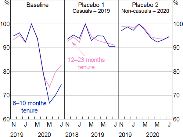
Sources: ABS; Authors' calculations
Unfortunately, the variable for the employee's status in employment (i.e. whether casual, permanent or self-employed) is only available in the LLFS from August 2014 onwards, which means we cannot not do a similar placebo test for the last major downturn – namely, the GFC in 2008–09.
D.4 Tenure Gradient in Employment Losses for Short-term Casuals
We also examined whether our baseline results are driven by last-in-first-out (LIFO) practices some firms may have used to prioritise dismissals during COVID-19. Specifically, longer-tenure casuals may have been more likely to retain their job than shorter-tenure casuals in the absence of JobKeeper, if firms tend to be more likely to dismiss their shorter-serving staff before their longer-serving staff during a downturn. Our baseline approach tries to circumvent this issue by restricting the estimation sample to a narrow range of tenure around the 12-month threshold. But for efficiency and data reasons, we still needed to include some people with modestly more tenure than others in our sample. The presence of LIFO practices may lead us to overstate the effect of JobKeeper on employment.
We test for this potential bias by examining whether short-term casuals with very short tenures (e.g. 1 or 2 months) in February 2020 were more likely to lose employment over the May to July period than short-term casuals with longer tenures (e.g. 9 or 10 months). To do this, we regress employment in a given month (say, July 2020) on the worker's tenure in their main job (a continuous variable) in February 2020. We do this for a sample of workers who were employed on a casual basis with between 1 and 10 months of tenure in February. All people in this group were ineligible for JobKeeper, so a positive and statistically significant ‘tenure gradient’ in employment would be evidence of LIFO practices. We find no statistically significant tenure gradient in May, June or July; indeed, in June and July the coefficient on the tenure variable has a negative sign, suggesting that, if anything, workers with more tenure were slightly less likely to remain employed than those with less tenure.[53]
D.5 Placebo Tests Using Non-casual Employees
We can also test for the presence of LIFO practices by looking at how employment rates of non-casual workers changed around the same tenure level as in our baseline approach. This is a useful exercise because non-casual workers are not subject to the 12-month tenure rule under JobKeeper, which means that any divergence in employment rates of non-casual workers around this threshold must be due to something other than the effects of JobKeeper, such as LIFO practices. We do not see any meaningful differences in the employment rates for non-casual employees with 6–10 months of tenure (in February 2020) relative to those with 12–23 months of tenure (Figure D1, right-hand panel). We take this as further evidence that any LIFO practices are not driving our baseline results.
The results of this placebo test also shed light on the role of firing costs, which can influence a firm's decisions to dismiss an employee when conditions deteriorate. In Australia, permanent employees are eligible for redundancy pay (a key component of firing costs) after 12 months of continuous service at a firm (FWO 2020c).[54] This means our placebo test using non-casual workers can be interpreted as a test both for LIFO effects and/or for the effects of higher firing costs on worker turnover (both effects are expected to operate in the same direction). As such, another interpretation of the placebo test result is that differences in firing costs are not important for explaining differences in employment outcomes across workers during the first few months of the COVID-19 crisis. Permanent employees eligible for redundancy pay did not have lower rates of job loss than those without it (Figure D1). However, this interpretation is muddied somewhat because the 12-month threshold for redundancy pay-eligibility is not anchored at a fixed point in time (unlike the threshold for JobKeeper eligibility which was anchored at 1 March), which means that some of the lower-tenure group became eligible for redundancy pay during the April to July 2020 period.
D.6 Excluding Multiple-job Holders
Our final robustness test is to examine if our results are sensitive to excluding multiple-job holders from the estimation sample. As discussed in Section 5.5, some individuals in our sample held more than one job prior to JobKeeper, but each person could only receive JobKeeper from their primary employer. Around 9 per cent of our treatment and control groups held more than one job in February 2020 (Table 1). In our baseline approach, we assigned individuals to the treatment and control groups based on the characteristics of their ‘main job’ in February.[55] There is not enough information in the LLFS on an individual's secondary job(s) to discern if those jobs were also worker-eligible for JobKeeper.
Our baseline estimates will understate the effect of JobKeeper worker eligibility on employment if some individuals in our control group were eligible for JobKeeper via their secondary job(s). One way to explore the extent of this bias is to re-estimate our models after excluding those who held more than one job prior to JobKeeper. This yields estimates of the effect of JobKeeper worker eligibility on employment that are 0.9 to 1.9 percentage points (or 10 to 20 per cent) larger than our baseline estimates during April to July. While this may suggest that some multiple-job holders in our control group did receive JobKeeper (and so our baseline estimates are biased downward), it may also reflect that multiple-job holders were less likely to have exited employment in the absence of JobKeeper.[56] In the LFS, a person remains ‘employed’ if they hold onto at least one of their jobs; all else being equal (and assuming that job losses are independent events), this is more likely to occur if a person had more jobs to begin with.[57] In other words, the treatment effect of JobKeeper on employment is plausibly smaller for multiple-job holders than for single-job holders because the former group were more likely to retain at least one job in the absence of JobKeeper. Again, it is worth reiterating that our analysis focuses on whether JobKeeper preserved employment, not jobs.
Appendix E: Alternative Identification Strategy
As a sense check on our baseline results, we also estimated the effects of JobKeeper on employment using a different component of the worker-eligibility test – the residency requirement. With the exception of New Zealand citizens, temporary residents were not eligible for JobKeeper.[58] This residency requirement provides us another way of estimating the causal effect of JobKeeper on employment.
E.1 Treatment and Control Groups
In this alternative approach, we focus entirely on differences in worker eligibility arising from the residency requirement, rather than the job tenure threshold used for our baseline results. As with the baseline approach, we begin by identifying two groups of workers that are similar aside from the fact that one of the groups does not meet the residency requirement and therefore cannot receive JobKeeper (the control group) and the other group does satisfy the residency test (treatment group). By comparing the average employment rates across these two groups before and after JobKeeper we can derive an estimate of the causal effect of JobKeeper on employment. As before, to do this we use person-level data from the LLFS and a difference-in-differences approach.
Specifically, we define the treatment group as workers who held a Subclass 444 (Special Category) Visa, notably citizens of New Zealand. Unlike other temporary visa holders, people on 444 visas are eligible for JobKeeper. The control group is recent arrivals on all other types of temporary visas, who are not eligible for JobKeeper.[59] Note that unlike our baseline approach, the treatment and control groups using the alternative identification strategy include a mix of casual and non-casual employees and self-employed.[60]
As the descriptive statistics in Table E1 show, recent arrivals from New Zealand are similar to recent arrivals from other countries in a number of ways, such as in the types of industries they tend to work in (in most cases). The main difference is that a smaller share of recent migrants from New Zealand were studying in Australia compared to those from other countries (and, as such, migrants from New Zealand also tend to be slightly older than other migrants, on average). We account for the differences in study patterns and age by controlling for these factors (and other factors) in our model directly.
| Control group (non-Oceanic born) | Treatment group (born in New Zealand or other Oceania) |
Difference | p-value of difference | |
|---|---|---|---|---|
| Industry (%) | ||||
| Agriculture, forestry & fishing | 2.6 | 0.0 | 2.6 | 0.2932 |
| Mining | 0.8 | 7.3 | −6.5 | 0.0003 |
| Manufacturing | 7.4 | 2.4 | 5.0 | 0.2306 |
| Electricity, gas, water & waste | 1.0 | 2.4 | −1.5 | 0.3853 |
| Construction | 6.1 | 4.9 | 1.2 | 0.7515 |
| Wholesale trade | 3.3 | 9.8 | −6.5 | 0.0340 |
| Retail trade | 12.9 | 7.3 | 5.5 | 0.3006 |
| Accomm & food services | 12.9 | 14.6 | −1.8 | 0.7425 |
| Transport, postal & ware | 7.4 | 12.2 | −4.8 | 0.2675 |
| Info media & telecom | 1.3 | 0.0 | 1.3 | 0.4603 |
| Finance & insurance | 1.8 | 4.9 | −3.1 | 0.1759 |
| Rental, hiring & real estate | 1.3 | 0.0 | 1.3 | 0.4603 |
| Prof, scientific & tech services | 12.5 | 2.4 | 10.1 | 0.0536 |
| Admin & support services | 5.8 | 9.8 | −4.0 | 0.2992 |
| Public admin & safety | 0.0 | 0.0 | 0.0 | na |
| Education & training | 4.1 | 4.9 | −0.8 | 0.8142 |
| Health care & social assistance | 13.5 | 7.3 | 6.2 | 0.2564 |
| Arts & recreation | 1.3 | 2.4 | −1.1 | 0.5535 |
| Other services | 4.0 | 7.3 | −3.4 | 0.2977 |
| Employment type (%) | ||||
| Casual | 33.4 | 36.6 | −3.1 | 0.6808 |
| Permanent | 55.4 | 63.4 | −8.1 | 0.3152 |
| Other | 11.2 | 0.0 | 11.2 | 0.0235 |
| Job tenure (years) | 1.8 | 1.9 | −0.1 | 0.7446 |
| Occupational skill level | 3.1 | 2.9 | 0.2 | 0.4928 |
| (1 = highest, 5 = lowest) | ||||
| Hours worked | 31.3 | 33.7 | −2.4 | 0.3080 |
| One job only (%) | 93.4 | 97.6 | −4.2 | 0.2914 |
| Student (%) | 24.5 | 12.2 | 12.4 | 0.0723 |
| Age (years) | 32.7 | 35.7 | −3.0 | 0.0216 |
| Female (%) | 42.7 | 53.7 | −11.0 | 0.1699 |
| Observations | 607 | 41 | ||
|
Note: Characteristics in February for sample remaining in June 2020; employees and self-employed who arrived in the past 1–6 years Sources: ABS; Authors' calculations |
||||
During the GFC, the rate of unemployment experienced by recent arrivals from New Zealand and the unemployment rate experienced by recent arrivals from other countries increased by a similar amount, suggesting these groups have similar sensitivity to changing economic conditions (Figure E1). This gives further confidence that labour market outcomes of these two groups would also have tracked quite closely during the COVID-19 period in the absence of JobKeeper. In contrast, Australian-born workers' outcomes are less sensitive to economic conditions, so using Australian-born as the treatment group would likely lead us to overstate the effects of JobKeeper on employment.
Notes:
Monthly data are smoothed using a 12-month trailing average
(a) Arrived in Australia within the past 1–6 years
Sources: ABS; Authors' calculations
E.2 Inferring Visa Status and Type
The LFS does not ask people whether they hold a visa or the type of visa they hold. But it does collect enough information to infer the likelihood a person holds a particular type of visa, if at all.[61] This includes:
-
Years since arrival
Survey and administrative data sources suggest that the longer a person lives in Australia, the more likely they are to be a citizen or permanent resident rather than a temporary resident (Figure E2).[62] This reflects the progression of temporary residents to permanent residency over time, and that those who do not attain permanent residency are more likely to leave the country.
Figure E2: Temporary Visa HoldersShare of foreign-born population, by years since arrival
Note: Excludes New Zealand citizens
Sources: ABS – Australian Census and Migrants Integrated Dataset, Australian Census and Temporary Entrants Integrated Dataset, and Characteristics of Recent Migrants Survey; Authors' calculations
We limit our estimation sample to migrants who arrived within the past 1–6 years (measured as of February 2020). The administrative data suggest that roughly half of all people who migrated to Australia within the past six years (and continue to live in Australia) are on a temporary visa, while the other half have attained permanent residency or citizenship (Figure E2). This means that our regression estimates – which pool over all people who arrived within the past 1–6 years regardless of their residency status – will underestimate the effect of JobKeeper by about one-half, all else being equal. We adjust for this bias by applying a scaling factor to our regression estimates (see Section E.4 below).
Our decision to focus on people who arrived in the past 1–6 years is designed to balance the trade-off between ensuring a large enough sample to estimate our regression coefficients precisely and diluting the share of the sample that actually hold a temporary visa.[63] We exclude those who arrived in the past 12 months because labour market outcomes of this group are volatile and unrepresentative.
-
Country of birth
To infer the type of visa a person holds, we use their country of birth as a proxy. Administrative data indicate that virtually all temporary residents born in New Zealand hold a 444 visa (ABS 2019a). The same is true for those born in other Oceanic countries, such as Samoa, the Cook Islands and Fiji, where 85 per cent of all temporary residents in Australia are on 444 visas (meaning they had New Zealand citizenship before migrating). In comparison, less than 10 per cent of temporary residents born outside the Oceanic region hold a 444 visa.[64]
We allocate migrants who arrived in the past 1–6 years to the treatment group if they were born in New Zealand or other Oceanic country, and to the control group if they were born elsewhere. Our estimation sample is restricted to those employed in February 2020, which means we implicitly focus on those with work rights.[65] We apply a (additional) scaling factor to our difference-in-differences estimates to account for the imperfect overlap between country of birth and whether a person holds a 444 visa or not (see Section E.4 below).
E.3 Estimation Equation
To estimate the effects of JobKeeper residency eligibility on employment we estimate a model similar to Equation (2), but replacing Eligi with a dummy variable that equals one if the worker was born in New Zealand or other Oceanic country, and zero if they were born elsewhere. We also include all the variables listed in Table E1 as controls (all of which are measured as of February 2020). We estimate this equation month-by-month using a linear probability model with robust standard errors.
E.4 Results
The top panel of Figure E3 shows the share of the treatment (dark line) and control group (light line) that were employed in each month between November 2019 and July 2020, conditional on being employed in February. Around 90¾ per cent of recently-arrived New Zealanders who were employed in February 2020 were still employed three months later, compared to 81½ per cent of those recent arrivals born in other countries. The difference in these employment rates in May – 9½ percentage points – is our difference-in-differences estimate for that month. These estimates are presented in the bottom panel of Figure E3, along with 95 per cent confidence intervals.
As discussed above, we need to apply a scaling factor to these regression estimates to account for the differences between the variables we observe in the data – country of birth and years since arrival – and what we would ideally observe – visa status and visa type. Applying this scaling factor (2.17) to our difference-in-differences estimates suggests that being worker-eligible for JobKeeper raised a person's probability of remaining employed by around 20 percentage points in May and 27 percentage points in June.[66] This is more than twice as large as the intent-to-treat effect we estimated using our baseline approach. The estimates for July were smaller and not statistically significant.
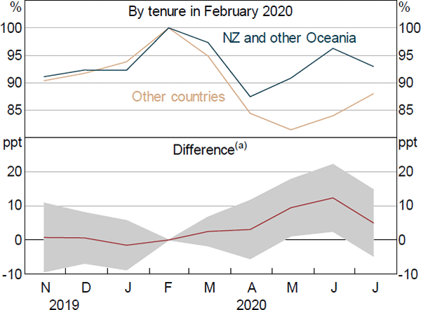
Notes:
Employees and self-employed who arrived in the past 1–6 years and were employed in February 2020; estimates conditional on the control variables listed in Table E1
(a) Shaded area represents 95 per cent confidence intervals
Sources: ABS; Authors' calculations
The implied effect of actually receiving JobKeeper on employment is also larger than our baseline estimate. To see this, we again assume that one-third of all worker-eligible individuals received JobKeeper.[67] This suggests that receiving JobKeeper increased a person's probability of staying employed by more than 60 percentage points in May and June, relative to the counterfactual of not receiving JobKeeper. This is three times larger than our baseline estimate. One possible explanation is that the effects of JobKeeper are heterogeneous, with JobKeeper being more effective at preserving employee-employer relationships within the population of recently arrived migrants than it was at preserving those relationships amongst permanent residents and citizens. However, the confidence intervals around this estimate are large (and likely larger than indicated on Figure 3).
It is reassuring that both identification strategies lead to the same overall conclusion that JobKeeper played a key role in cushioning employment losses in its first four months. In both cases, the point estimates are economically and statistically significant, they just differ in magnitude.
Although the migration approach provides a useful sense check, our overall assessment about the quantitative effect of JobKeeper on total employment is based on our preferred approach using the tenure eligibility of casuals. We have more confidence in the results from our baseline approach, as it has fewer potential issues than the migration approach (discussed below). If we had placed more weight on the migration approach, our headline estimate of the employment effect of JobKeeper would be larger.
E.5 Limitations
Relative to our baseline approach (using the 12-month tenure rule for casual workers), the alternative identification strategy has several shortcomings that explain why we give it less emphasis:
- Sample size: there are only 53 individuals in the treatment group (801 in the control group) for estimating the employment effect in May.[68] There is a risk that our IV-style estimator suffers from a small sample bias.
- Adjustments for incomplete data: imperfect measures of visa status and visa type mean we need to make adjustments to our regression estimates that can introduce error. Also, the standard errors do not account for these adjustments, so the precision of our estimates is likely overstated.
- Parallel trends: the treatment and control groups are far less balanced on observable dimensions than in the baseline approach (Table E1). Although we control for these variables in our model, this lack of balance on observables suggests a greater risk that the treatment and control groups will also differ in terms of unobservable factors associated with employment loss. Indeed, there is some evidence of an ‘effect’ of JobKeeper before the program was announced (Figure E3, albeit not statistically significant), which may signal a violation of the parallel trends assumption.
- External validity: recent migrants are likely less representative of the broader population of JobKeeper recipients than the casual sample used for the baseline results. For example, most recent migrants do not have access its other forms of income support, such as the JobSeeker payment, which could influence their responses.
- Selection bias: our estimates may be biased if temporary visa holders departed Australia (and thus drop out of our sample) if their work prospects were adversely affected by COVID-19.[69] The number of visa holders from New Zealand remained fairly steady during the COVID-19 crisis, while those from all other countries have fallen sharply (Figure E4).
Note: (a) Temporary skilled, student, temporary graduate and working holiday maker visa
Sources: Authors' calculations; Department of Home Affairs
E.6 Differential Treatment Effects by Employment Type
Although our main approach is restricted to casual employees, the migration approach captures the effects of JobKeeper on both casual and permanent staff, and also the self-employed. The estimates in Figure E3 restrict the effects of JobKeeper worker eligibility to be constant across these different categories of employment. Relaxing this assumption allows us to test whether the effects of JobKeeper worker eligibility differs for casuals and permanent employees.[70]
To investigate this further we augment our model with an interaction between the treatment variable and a dummy variable that equals one if the worker is a permanent employee, and zero otherwise.[71] A test for differential effects for employees on different work arrangements is a test of whether the coefficient on this interaction is statistically significant. The coefficient is close to zero and not significant (p-value = 0.66, 0.64 and 0.31 in May, June and July). That is, we cannot reject the hypothesis that the effects of JobKeeper on casuals and permanent employment are equal. We discussed this finding in Section 8.3. An issue with this test is that it is based on a very small sample (particularly at the subgroup level), so has low power.
References
Abraham KG and SN Houseman (2014), ‘Short-Time Compensation as a Tool to Mitigate Job Loss? Evidence on the U.S. Experience during the Recent Recession’, Industrial Relations, 53(4), pp 543–567.
ABS (Australian Bureau of Statistics) (2015), ‘Leave Entitlements Data from the Labour Force Survey’, ‘Labour Force, Australia, Detailed, Quarterly’, November, ABS Cat No 6291.0.55.003, viewed 29 October 2020. Available at <https://www.abs.gov.au/ausstats/abs@.nsf/Previousproducts/6291.0.55.003Main%20Features6Nov%202015?opendocument&tabname=Summary&prodno=6291.0.55.003 &issue=Nov%202015&num=&view=>.
ABS (2017), ‘Australian Labour Account Concepts’, ‘Australian Labour Account: Concepts, Sources and Methods, 2017’, ABS Cat No 6150.0, pp 17–30.
ABS (2018), ‘The Labour Force Framework’, ‘Labour Statistics: Concepts, Sources and Methods, 2018’, ABS Cat No 6102.0.55.001, pp 35–52.
ABS (2019a), ‘Insights from the Australian Census and Temporary Entrants Integrated Dataset’, viewed 29 October 2020. Available at <https://www.abs.gov.au/statistics/people/people-and-communities/insights-australian-census-and-temporary-entrants-integrated-dataset/latest-release>.
ABS (2019b), ‘Jobs in Australia, 2011-12 to 2016-17’, ABS Cat No 6160, accessed 29 October 2020. Available at <https://www.abs.gov.au/AUSSTATS/abs@.nsf/Lookup/6160.0Main+Features12011-12%20to%202016-17?OpenDocument>.
ABS (2020a), ‘Business Indicators, Business Impacts of COVID-19’, April, viewed 29 October 2020. Available at <https://www.abs.gov.au/statistics/economy/business-indicators/business-indicators-business-impacts-covid-19/apr-2020>.
ABS (2020b), ‘Employment and Unemployment: An International Perspective’, ‘Labour Force, Australia’, August, viewed 29 October 2020. Available at <https://www.abs.gov.au/articles/employment-and-unemployment-international-perspective>.
ABS (2020c), ‘Secondary Jobs around 30 per cent of Total Payroll Job Losses’, ‘Weekly Payroll Jobs and Wages in Australia’, Week ending 8 August, viewed 29 October 2020. Available at <https://www.abs.gov.au/statistics/labour/earnings-and-work-hours/weekly-payroll-jobs-and-wages-australia/week-ending-8-august-2020#secondary-jobs-around-30-per-cent-of-total-payroll-job-losses>.
ABS (2020d), ‘Survey Impacts and Changes: Treatment of People on JobKeeper, JobSeeker or Stood Down’, ‘Labour Force, Australia’, August, viewed 29 October 2020. Available at <https://www.abs.gov.au/statistics/labour/employment-and-unemployment/labour-force-australia/aug-2020>.
Angrist JD and J-S Pischke (2009), Mostly Harmless Econometrics: An Empiricist's Companion, Princeton University Press, Princeton.
ATO (Australian Taxation Office) (2020a), ‘Partnerships, Trusts and Companies’, JobKeeper Payment, ATO website, viewed 29 October 2020. Available at <https://www.ato.gov.au/General/JobKeeper-Payment/Partnerships,-trusts-and-companies/>.
ATO (2020b), ‘Step 1: Enrol for the JobKeeper Payment’, JobKeeper Payment, ATO website, viewed 29 October 2020. Available at <https://www.ato.gov.au/General/JobKeeper-Payment/In-detail/JobKeeper-guide---employers-reporting-through-STP/?page=2#Step_1__Enrol_for_the_JobKeeper_payment>.
Australian Government (2020a), ‘Budget Paper No. 1: Budget Strategy and Outlook 2020–01’.
Australian Government (2020b), ‘COVID-19 Response: Supporting Australians through the Crisis’, Budget 2020-21, viewed 29 October 2020. Available at <https://budget.gov.au/2020-21/content/covid-19.htm>.
Australian Government (2020c), ‘Economic and Fiscal Update: July 2020’.
Autor D, D Cho, LD Crane, M Goldar, B Lutz, J Montes, WB Peterman, D Ratner, D Villa and A Yildirmaz (2020), ‘An Evaluation of the Paycheck Protection Program Using Administrative Payroll Microdata’, Unpublished manuscript, 22 July.
Balleer A, B Gehrke, W Lechthaler and C Merkl (2016), ‘Does Short-Time Work Save Jobs? A Business Cycle Analysis’, European Economic Review, 84, pp 99–122.
Bartik AW, M Bertrand, F Lin, J Rothstein and M Unrath (2020), ‘Measuring the Labor Market at the Onset of the COVID-19 Crisis’, NBER Working Paper No 27613.
Bishop J, L Gustafsson and M Plumb (2016), ‘Jobs or Hours? Cyclical Labour Market Adjustment in Australia’, RBA Research Discussion Paper No 2016-06.
Boeri T and H Bruecker (2011), ‘Short-Time Work Benefits Revisited: Some Lessons from the Great Recession’, Institute for the Study of Labor, IZA Discussion Paper No 5635.
Burda MC and J Hunt (2011), ‘What Explains the German Labor Market Miracle in the Great Recession?’, Brookings Papers on Economic Activity, Spring, pp 273–319.
Cassells R and A Duncan (2020), ‘JobKeeper: The Efficacy of Australia's First Short-Time Wage Subsidy’, Australian Journal of Labour Economics, 23(2), pp 99–128.
Chetty R, JN Friedman, N Hendren, M Stepner and The Opportunity Insights Team (2020), ‘How Did COVID-19 and Stabilization Policies Affect Spending and Employment? A New Real-Time Economic Tracker Based on Private Sector Data’, NBER Working Paper No 27431.
Department of Home Affairs (2018), ‘Temporary Visa Holders in Australia’, accessed 29 October 2020. Available at <https://data.gov.au/dataset/ds-dga-ab245863-4dea-4661-a334-71ee15937130/details?q=>.
Efstathiou K, TY Mathä, C Veiga and L Wintr (2018), ‘Short-Time Work in Luxembourg: Evidence from a Firm Survey’, Journal for Labour Market Research, 52, Article 14.
Frydenberg J (Treasurer) (2020), ‘JobKeeper Payment Supporting Millions of Jobs’, Media Release, 14 April. Available at <https://ministers.treasury.gov.au/ministers/josh-frydenberg-2018/media-releases/jobkeeper-payment-supporting-millions-jobs>.
FWO (Fair Work Ombudsman) (2020a), ‘Casual Employees’, Employee Entitlements, FWO website, viewed 29 October 2020. Available at <https://www.fairwork.gov.au/employee-entitlements/types-of-employees/casual-part-time-and-full-time/casual-employees>.
FWO (2020b), ‘Ending Employment & the JobKeeper Scheme’, Coronavirus and Australian Workplace Laws, FWO website, viewed 29 October 2020. Available at <https://coronavirus.fairwork.gov.au/coronavirus-and-australian-workplace-laws/pay-and-leave-during-coronavirus/jobkeeper-wage-subsidy-scheme/ending-employment-and-the-jobkeeper-scheme>.
FWO (2020c), ‘Notice of Termination & Redundancy Pay’, How will we Help, FWO website, viewed 29 October 2020. Available at <https://www.fairwork.gov.au/how-we-will-help/templates-and-guides/fact-sheets/minimum-workplace-entitlements/notice-of-termination-and-redundancy-pay>.
Granja J, C Makridis, C Yannelis and E Zwick (2020), ‘Did the Paycheck Protection Program Hit the Target?’, NBER Working Paper No 27095.
Hamilton S (2020), ‘A Tale of Two Wage Subsidies: The American and Australian Fiscal Responses to COVID-19’, George Washington University, Elliot School of International Affairs, Institute for International Economic Policy Working Paper IIEP-WP-2020-12.
Hijzen A and S Martin (2013), ‘The Role of Short-Time Work Schemes during the Global Financial Crisis and Early Recovery: A Cross-Country Analysis’, Institute for the Study of Labor, IZA Discussion Paper No 7291.
Hubbard G and MR Strain (2020), ‘Has the Paycheck Protection Program Succeeded?’, Paper presented at the Brookings Papers on Economic Activity Fall Conference ‘COVID-19 and the Economy’, Online, 24 September.
Kopp D and M Siegenthaler (2018), ‘Does Short-Time Work Prevent Unemployment?’, Swiss Economic Institute, KOF Studies No 106.
Lydon R, TY Mathä and S Millard (2018), ‘Short-Time Work in the Great Recession: Firm-Level Evidence from 20 EU Countries’, Central Bank of Ireland Research Technical Paper, 2018(13).
Migrant Workers' Taskforce (2019), Report of the Migrant Workers' Taskforce, (A Fels, Chair), March, Australian Government, Canberra.
Möller J (2010), ‘The German Labor Market Response in the World Recession – De-mystifying a Miracle’, Journal for Labour Market Research, 42(4), pp 325–336.
Morrison S (Prime Minister) and J Frydenberg (Treasurer) (2020), ‘More Support for More Businesses and Workers’, Joint Media Release, 7 August.
OECD (Organisation for Economic Co-operation and Development) (2020), ‘Issue Note 5: Flattening the Unemployment Curve? Policies to Support Workers' Income and Promote a Speedy Labour Market Recovery’, OECD Economic Outlook, 2020(1), No 107, pp 114–129.
RBA (Reserve Bank of Australia) (2020), ‘Box A: Using Wage Subsidies to Support Labour Markets through the COVID-19 Shock’, Statement on Monetary Policy, August, viewed 29 October 2020. Available at <https://www.rba.gov.au/publications/smp/2020/aug/box-a-using-wage-subsidies-to-support-labour-markets-through-the-covid-19-shock.html>.
Treasury (Australian Treasury) (2020a), ‘JobKeeper Payment — Information for Employers’, Economic Response to the Coronavirus, Fact Sheet, 9 June.
Treasury (2020b), ‘The JobKeeper Payment: Three-Month Review’, June.
Treasury and ATO (2020), ‘JobKeeper Update’, Joint Media Release, 22 May.
Copyright and Disclaimer Notice
HILDA Survey Disclaimer
This paper uses unit record data from the Household, Income and Labour Dynamics in Australia (HILDA) Survey. The unit record data from the HILDA Survey was obtained from the Australian Data Archive, which is hosted by The Australian National University. The HILDA Survey was initiated and is funded by the Australian Government Department of Social Services (DSS) and is managed by the Melbourne Institute of Applied Economic and Social Research (Melbourne Institute). The findings and views based on the data, however, are those of the authors and should not be attributed to the Australian Government, DSS, the Melbourne Institute, the Australian Data Archive or The Australian National University and none of those entities bear any responsibility for the analysis or interpretation of the unit record data from the HILDA Survey provided by the authors.
Acknowledgements
For helpful comments and suggestions we thank Natasha Cassidy, Iris Chan, Nathan Deutscher, Pauline Grosjean, Jonathan Hambur, Gabrielle Penrose, John Simon, Lachlan Vass, Luke Willard and seminar participants at the Reserve Bank of Australia and Australian Treasury. We would like to thank the Australian Bureau of Statistics for making the LFS microdata data available to us, and in particular to Scott Marley for his assistance. The views expressed in this paper are those of the authors and do not necessarily reflect the views of the Reserve Bank of Australia. The authors are solely responsible for any errors. Our programs and publicly available data are available at <https://www.rba.gov.au/publications/rdp/2020/2020-07/supplementary-information.html>.
Footnotes
The 3.5 million figure is based on Treasury's (2020b) estimate for May 2020 and more recent reports in the Budget (Australian Government 2020a, p 1-13) (these are point-in-time figures). The budget papers also noted that more than 3.8 million people have received the JobKeeper payment at some point since the program's inception. [1]
This amount is close to the national minimum wage for full-time employees ($1,481.60 per fortnight). [2]
The first of these ATO payments to eligible firms were made in arrears in the first week of May, and then on a monthly cycle thereafter. [3]
The New Zealand wage subsidy scheme has different payment rates for full-time and part-time workers. Cassells and Duncan (2020) emphasise the uniqueness of the flat payment rate. The authors note that ‘[o]f the more than fifty countries that have introduced emergency wage subsidies over the course of the pandemic, none paid a single rate to all eligible workers regardless of their normal wage or employment status’ (p 109). [4]
Hamilton (2020) argues that the flat per-worker subsidy undercompensates businesses for their higher earners, and the wage floor prevents them from being overcompensated for their lower earners. Cassells and Duncan (2020) note that most international wage subsidy schemes impose a floor on the amount an employer must pay an employee, normally a fraction (below 1) of the employee's usual wage. [5]
Revenue is on a consolidated basis, so includes the revenue of any individual or business affiliated with the entity. Self-employed individuals were eligible to receive the JobKeeper Payment where they met the relevant turnover test. There were also some additional restrictions on eligibility; for example, public sector agencies and entities subject to the Major Bank Levy were ineligible (ATO 2020a). [6]
On 7 August 2020, it was announced that from 3 August 2020 the relevant date of employment for assessing eligibility would move from 1 March to 1 July 2020, expanding employee eligibility for the existing scheme and the extension. [7]
An ABS (2020a) survey in late April revealed that 90 per cent of eligible firms (with at least some eligible employees) had enrolled in the program or were intending to do so. The reasons firms cited for not enrolling included insufficient cash flow to continue paying workers until the JobKeeper payments commence (23 per cent), difficulty understanding the eligibility criteria (23 per cent) and ‘other’ reasons (54 per cent). [8]
An employer could dismiss an employee receiving JobKeeper by following the usual process for ending employment (FWO 2020b). [9]
Data from ABS (2019a) and the 2016 Australian Census indicated that temporary residents accounted for around 18 per cent of total employment in the accommodation & food services industry in 2016, which was the highest employment share of any industry. [10]
The PPP extends forgivable loans to small businesses, via private banks. The forgiveness is achieved by maintaining employment at pre-COVID-19 levels, which means PPP loans constitute an implicit wage subsidy (Hamilton 2020). [11]
There are exceptions, such as Canada's scheme. [12]
Casual employment status is inferred based on the reported absence of paid leave entitlements (either paid holiday leave or paid sick leave). According to the ABS (2015), this is ‘the most objective and commonly used measure of casual employment’. [13]
In Appendix D.6, we show that our results are unlikely to be materially affected by our focus on main jobs rather than both main and second jobs. [14]
If a person did not pass the worker-eligibility test in their main job, they may still have passed in a second job. We discuss this in Appendix D.6, along with the results of a robustness test that suggests this does not create a material bias. [15]
Some people who were JobKeeper worker-eligible in their main job may not have received the JobKeeper payment for that job if they instead received the payment for a job that was not their main job. But, in that case, the person still received JobKeeper. The individual's main job (as defined in the LFS) can differ from their primary employer (as defined by the ATO). [16]
Table C1 compares the descriptive statistics in Table 1 with equivalent descriptive statistics for the sample of all casual employees in February 2020 (including those with less than 6 months of tenure or more than 23 months of tenure) and the sample of all employees in February 2020 (including all casual and non-casual employees). [17]
An alternative approach would be to control for these pre-treatment differences directly (interacted with the time dummy). However, introducing control variables will only account for observable differences between the treatment and control groups, not the unobservable differences that may have affected employment outcomes in the absence of JobKeeper. [18]
In Appendix D.4, we present evidence that an employee's job tenure as at February 2020 was not predictive of his or her probability of remaining employed over the May to July period, for those people with 1 to 10 months tenure. This suggests that our baseline results would be robust to varying the width of the tenure window on the left-hand side of the 12-month cut-off. [19]
Some key awards that include this provision include the Hospitality Industry (General) Award [MA000009], Fast Food Industry Award [MA000003], General Retail Industry Award [MA000004], Hair and Beauty Industry Award [MA000005] and the Real Estate Industry Award [MA000106]. What constitutes ‘reasonable grounds’ to refuse the request varies by award, but can include: the employee does not work regular hours, the employee's job will not exist in the next 12 months, or the employee's working hours will be significantly reduced in the next 12 months. In other awards, a casual conversion request can be made after 6 months, such as the Manufacturing and Associated Industries and Occupations Award [MA000010] and the Building and Construction General On-site Award [MA000020]. [20]
The 12-month threshold for requesting flexible work arrangements, unpaid parental leave or permanent employment is not anchored at a fixed point in time (unlike the threshold for JobKeeper eligibility which was anchored at 1 March), which means that some of the lower-tenure group became eligible for these options during the April to July 2020 period. [21]
The key identifying assumptions of RDD are likely to be satisfied in that there was very limited scope for employers to manipulate the job tenure information given to authorities (see Section 2.3). Using these other datasets it may also be possible to exploit discontinuities in the revenue decline cut-offs in the firm-eligibility test. In saying that, the revenue decline cut-offs were fuzzier than the cut-offs that applied to individual workers, particularly given that firm eligibility could be based on projected, rather than actual, revenue losses, and that alternative tests could also apply. [22]
The LLFS micro data does not include a variable for whether the employee works in the public sector, so instead we drop employees in 3-digit industries where more than 60 per cent of employees are employed in the public sector (based on data from the 2016 Census). In addition to all industry sub-groups within the Public Administration & Safety industry division, this includes employees working in hospitals, tertiary education, rail and some utilities. The LLFS micro data does not identify whether the employee works for a major bank, so we drop any employees who works in the 3-digit Depository Financial Intermediation industry. Industry in the LLFS pertains to the individual's main job. [23]
By June, there were 377 people in the treatment group and 274 people in the control group. By July, there were 273 in the treatment group and 189 in the control group. More than two-thirds of people in February 2020 had left the panel by July. Much of this sample loss reflects the 8-month rotating panel design of the LFS, which reduces the initial sample by roughly one-eighth for every month we extend our analysis into the future. By July, sample rotation accounts for over 90 per cent of all exits from the survey panel relative to February, while premature attrition (attrition not explained by rotation) accounts for the remainder. While sample rotation leads to some data being ‘missing at random’, a potential source of bias in our study is the possibility that premature attrition does not occur at random. While our treatment and control groups are balanced across many of the observable dimensions that tend to be associated with attrition (e.g. age, occupational skill level), it is possible that premature attrition is also correlated with changes in a person's employment status, and if so, it can create a bias in our regression estimates. One source of premature attrition happens when households change their address, because the ABS drops those households from the survey. Because regional mobility is often associated with a change in employment status (e.g. a person who loses their job may relocate to a new region to find work), this non-random premature attrition could lead to a bias in our estimates. However, during COVID-19 this ‘mobility bias’ is likely to be smaller than normal, due to the constraints on moving home during the pandemic. In July, the premature attrition rates were higher for our control group (8.2 per cent of the February control group sample) than for our treatment group (5.7 per cent of the February treatment group sample). As such, if we assume those who prematurely left the panel did so as a result of job loss, our estimates of the effect of JobKeeper on employment would be understated. Indeed, if all the people who prematurely left the survey panel did so because of job loss, adjusting our difference-in-differences estimates to account for this (by setting the employment status of all premature leavers to ‘non-employed’ rather than ‘missing’) would yield estimates of the effect of JobKeeper worker eligibility on employment equal to 12.9 percentage points, which is higher than our baseline estimate of 8.2 percentage points (Figure 2). The bias will run in the opposite direction if premature attrition is negatively associated with employment. [24]
These changes were announced on 7 August 2020 and effective from 3 August. The August LFS referenced the period 1–15 August. [25]
A person who is not employed can either be unemployed or not in the labour force. We do not distinguish these states. [26]
We are being loose with our terminology here. Our difference-in-differences estimate actually yields the effect of JobKeeper tenure eligibility. This is slightly different to the effect of worker eligibility because the latter also requires the worker meet the residency requirement. [27]
Clustering the standard errors at the 2-digit ANZSIC 2006 industry level (at least 52 clusters over May to July 2020) produced standard errors that were 26 per cent (May), 18 per cent (June) and 6 per cent (July) smaller than robust standard errors that do not allow for intra-industry correlation. As such, our decision to use robust, rather than cluster-robust, standard errors is conservative. [28]
This is consistent with the long-standing concepts and practices used in the LFS. For more information, see ABS (2020d). [29]
The ABS payroll data suggest that the number of secondary jobs fell sharply relative to main jobs during our period of analysis (ABS 2020c). In Appendix D.6, we provide some discussion on the effects of multiple job holding on our results. [30]
Table C2 provides the month-by-month regression estimates of Equation (2) in table format. [31]
This lag occurs for two reasons. First, the survey asks about a given reference week. A worker who loses their job midway through that week is classified as employed if they worked at least one hour at the start of the week. This is important for interpreting the April survey, because a number of high-frequency data sources suggest a large amount of job shedding occurred during the reference weeks of the April LFS. There is also evidence for this in the sharp rise in the number of people reporting fewer than their usual hours during the April reference week(s) because they ‘lost or left a job’ during that week. These job losses did not flow through to employment until May. Second, people who are stood down without pay continued to be classified as employed for at least four weeks after being stood down (see Section 5.5). While this treatment of unpaid stand downs is consistent with the best-practice guidelines set out by the International Labour Organization, it differs to the treatment in Canada and the United States where such layoffs lead to an immediate decline in employment. [32]
Future work using administrative data should seek to better understand the relationship between eligibility and take-up across different employment types (e.g. casual or non-casual) and different ranges of job tenure. [33]
See the business case study on page 28 of Treasury (2020b). [34]
Another consideration is the effects of cross-subsidisation coming from infra-marginal employees at the firm who received JobKeeper (e.g. eligible casual employees at the firm with more than two years of job tenure or eligible permanent employees). However, there is no clear reason to believe that this cross-subsidisation effect should be any larger for our control group than for our treatment group. [35]
When thinking about the substitution effect of the JobKeeper Payment program, we abstract from the income effect of the JobKeeper Payment program itself but not the adverse shock to firm incomes caused by the COVID-19 crisis. [36]
The latter group comprises those who have been stood down for more than four weeks without pay. [37]
Treasury (2020b) analysis of business micro data suggests that in the fortnight ending 24 May 400,000 people were stood down on JobKeeper, or around 11½ per cent of all recipients. This is consistent with our analysis of the LLFS micro data, which suggests that in May around 310,000 people were classified as ‘away from work’ for more than four weeks but still being paid by their employer. The small discrepancy between the Treasury's estimate and our own estimate based on the LLFS may reflect that our estimate excludes any stood down JobKeeper recipients who also held a second job or who found work at another firm. [38]
If the effect of JobKeeper worker eligibility on employment and total hours is 7 per cent and 5 per cent respectively, the effect on average hours worked is approximately –2 per cent. [39]
The confidence intervals in Figure 1 reflect the confidence intervals on our estimates of the effect of worker eligibility and do not account for the uncertainty related to our estimate of the take-up rate discussed in Section 6.2. [40]
Treasury estimated the unemployment rate would peak at 10 per cent with JobKeeper and 15 per cent without JobKeeper (Frydenberg 2020). This ex ante estimate was not affected by the revelation of a reporting error in estimates of the number of employees likely to access the program (and associated budget costing revisions) announced in May (Treasury and ATO 2020). [41]
The implied amount of employment saved by Treasury's estimate will be larger than 700,000 if some of those who exit employment are assumed to leave the labour force rather than becoming unemployed. [42]
The PPP funds could fully cover a firm's pre-COVID payroll expenses for 10 weeks, or one-quarter of their pre-COVID payroll expenses for 24 weeks (or anywhere in between). [43]
In most awards, casual employees are required to be paid an hourly wage premium, which helps to at least partly compensate for the loss of other benefits. [44]
The choice of employment relationship is also endogenous to the value of the worker-firm match. Casual and permanent employees may also have different levels of productivity, firm-specific human capital and wages. [45]
Data from the HILDA Survey suggests that 83 per cent of casuals with at least 12 months of job tenure who were working in the industries most adversely affected by COVID-19 (namely store-based retailing excluding food & fuel, arts & recreation, accommodation & food services, and other services) would have had their pre-scheme earnings more than fully covered by JobKeeper (i.e. a replacement ratio equal to 1 or more), compared to only 31 per cent of non-casual employees. This calculation assumes all employees received wage increases of 3 per cent per year between late 2017 and late 2019. [46]
For a discussion of the role of workplace-level flexibility in how the labour market adjusts to shocks, see Bishop et al (2016). [47]
In this simplified model, the revenue measure excludes any revenue from the JobKeeper subsidy itself. There are likely other worker- and firm-level variables we need to control for in Model (B1) to get an unbiased estimate of , but for expositional simplicity we assume that all relevant confounders are captured by the Revenuei,f,j variable. [48]
We do not adjust for visa status because we did not exclude temporary visa holders from the estimation sample for Equation (2). [49]
The notion that the numerator and denominator of Equation (B3) do not need to come from the same sample is based on the two-sample IV (TSIV) estimator (see Angrist and Pischke (2009, pp 147–148)). [50]
E(JobKeeperi|Eligi = 1) , where k denotes 1-digit ANZSIC 2006 industry division. The number of JobKeeper recipients by industry is from Treasury (2020b, p 43), which we adjust (proportionally) so that industry totals sum to 3.5 million. [51]
Our IV approach yields a local average treatment effect (LATE) – that is, the effect of JobKeeper on employment for those whose treatment status (receiving JobKeeper) is affected by worker eligibility. Always-takers do not exist in our set-up because a worker could not receive JobKeeper if they were not worker-eligible. For this reason, the LATE also corresponds to the ATT (Angrist and Pischke 2009, p 160). [52]
The p-values on the tenure coefficient in May, June and July are 0.14, 0.86 and 0.62, respectively. [53]
After one year, the employee is entitled to four weeks of pay at their base pay rate in the event of being made redundant. The generosity of these redundancy payments increases with every additional year of service up to ten years (FWO 2020c). [54]
In the LFS, an individual's main job is the job in which they usually work the most hours. [55]
Part of the difference might also reflect that multiple-job holders in our treatment group were more likely to receive JobKeeper than single-job holders in our treatment group, to the extent that they were also worker-eligible in their secondary jobs. [56]
Our analysis of ABS data for 2016/17 (ABS 2019b) suggests that two-thirds of multiple job holders who worked in one of the industries that were most adversely affected by COVID-19 (i.e. hospitality, arts, retail, real estate or other services) were partly ‘insured’ against the shock as they also held a second job in one of the less-affected industries. [57]
To be eligible for JobKeeper, a person must have been an Australian citizen or have held a permanent visa or Special Category (Subclass 444) Visa (and were a resident for Australian tax purposes) as at 1 March 2020 (Treasury 2020a). [58]
As at 30 March, there were 965,000 temporary visa holders with a right to work in Australia (excluding New Zealand citizens), of which 59 per cent were students. The remainder of those with work rights held a working holiday maker, temporary skilled, or temporary graduate visa. These data are from the Department of Home Affairs (2018). Not all visa holders with a work right will exercise that right, especially partners and children of a primary visa holder. These figures include secondary visa holders (i.e. family members), who typically also have work rights. Temporary visa holders with a work right are entitled to the same basic rights and protections as Australian citizens and permanent residents under Australian workplace laws (Migrant Workers' Taskforce 2019). Student visa holders are limited to working a maximum of 40 hours per fortnight during teaching periods, and unlimited hours during vacation periods. [59]
We exclude from the sample any worker employed in the public sector or for a major bank. [60]
The LFS only collects data on usual residents of Australia, which means the survey excludes overseas visitors. The official ABS definition of a usual resident is a person who has been (or expects to be) residing in Australia for 12 months or more in a 16-month period. However, the LFS uses a less precise approach; a screening question simply asks if the respondent is a short-term resident and, if so, they are excluded from the survey (ABS 2017). This criterion is based on a person's duration of stay within Australia. [61]
There are differences in the scope of these collections. The Census excludes those who indicated they would be usually resident in Australia for less than one year (‘overseas visitors’). [62]
Unlike other temporary migrants, New Zealand citizens who have lived in Australia for at least 10 years without interruption are eligible for JobSeeker for up to 6 months. Excluding people who have resided in Australia for more than 10 years means we will not accidentally attribute the effects of some other policy (e.g. JobSeeker) to JobKeeper. [63]
The share of temporary residents on 444 visas is relatively high for those born in the United Kingdom (28 per cent) and South Africa (54 per cent). [64]
Clearly some people in Australia without work rights may still seek work in the underground economy. However, after accounting for the screening questions in the LFS, it is unlikely that migrants working illegally represent a material share of our estimation sample. [65]
This scaling factor is calibrated using data from external administrative and survey sources. It accounts for the share of recent arrivals that are temporary, rather than permanent (around 52 per cent) and also a small adjustment for the fact that a small share of the control group also hold a 444 visa (around 6 per cent). This implies that 46 per cent of our control group is likely to be definitely ineligible for JobKeeper based on their residency status. In turn, this means we need to scale our resulting difference-in-differences estimate by 2.17 (= 1 ÷ 0.46) in order to get an intent-to-treat effect that is consistent with the intent-to-treat effect estimated using the baseline approach. This scaling factor is different to the scaling factor needed to translate our estimates of the effect of worker eligibility to estimates of the effect of JobKeeper. [66]
The take-up rate is close to ⅓ when we stratify the take-up rate calculation by the industry composition of the recent migrant sample. [67]
In June there are 41 and 607 individuals in the treatment and control groups, respectively, and 31 and 423 in July. [68]
Even if our treatment and control groups had experienced similar COVID-19 shocks overall, this non-random attrition from the sample would lead us to understate the effects of JobKeeper on employment amongst those who remained in the sample. However, to the extent that this fall was driven by border closures preventing re-entry of foreigners, rather than because of increased exits due to labour market conditions, this attrition need not be a source of bias. Our sample is matched, meaning that students who did not return to Australia for study in early 2020 are not included anyway. [69]
Casual and permanent employees may also have different levels of productivity, firm-specific human capital and wages. [70]
The base category is casual employees. We also include interactions for ‘other’ employment types (self-employed and contributing family workers) and the main effects. [71]