Research Discussion Paper – RDP 2019-03 Online Appendix: Explaining Monetary Spillovers: The Matrix Reloaded
This appendix provides additional information to accompany Research Discussion Paper No 2019-03. Section 1 provides a data overview. Section 2 provides some supplementary figures and tables.
1. Data Overview
| Advanced (27) | Emerging market (20) | |||||
|---|---|---|---|---|---|---|
| Euro area | Other | Asia | Europe | Latin America | Other | |
| Austria | Australia | China | Poland | Brazil | Nigeria | |
| Belgium | Canada | India | Romania | Chile | Pakistan | |
| Finland | Czech Republic | Indonesia | Turkey | Colombia | Russia | |
| France | Denmark | Malaysia | Mexico | South Africa | ||
| Germany | Hong Kong | Philippines | Peru | |||
| Greece | Israel | Thailand | Venezuela | |||
| Ireland | Japan | Vietnam | ||||
| Italy | New Zealand | |||||
| Netherlands | Norway | |||||
| Portugal | Singapore | |||||
| Spain | South Korea | |||||
| Sweden | ||||||
| Switzerland | ||||||
| Taiwan | ||||||
| United Kingdom | ||||||
| United States | ||||||
| Variable | Description | Source |
|---|---|---|
| Interest rates | ||
| 1-month and 6-month OIS | Overnight indexed swaps | Bloomberg; Thomson Reuters Tick History |
| 2-year and 10-year bond yields | Sovereign bond yields | Bloomberg; Thomson Reuters Tick History |
| Global controls | ||
| US 10-year yield | Sovereign benchmark bond yield | |
| VIX | S&P 500 volatility index | Bloomberg |
| Economic conditions | ||
| Real GDP | Year-ended growth | BIS; OECD; IMF World Economic Outlook |
| CPI inflation | Annual rate | BIS; IMF International Financial Statistics |
| Bilateral trade | Imports and exports of goods and services between originator and recipient economy, ratio to GDP | IMF Direction of Trade Statistics |
| Common language | Dummy equals one if originator and recipient share a common language | Mayer and Zignago (2011) |
| Weighted distance | Distance between originator and recipient | Mayer and Zignago (2011) |
| Time difference | Time difference between originator and recipient | Mayer and Zignago (2011) |
| Financial openness | ||
| Portfolio equity | Stock of recipient economy (total assets or liabilities) as a ratio to GDP | Lane and Milessi-Ferretti (2017) |
| Portfolio debt | Stock of recipient economy (total assets or liabilities) as a ratio to GDP | Lane and Milessi-Ferretti (2017) |
| FDI (foreign direct investment) | Stock of recipient economy (total assets or liabilities) as a ratio to GDP | Lane and Milessi-Ferretti (2017) |
| Financial derivatives | Stock of recipient economy (total assets or liabilities) as a ratio to GDP | Lane and Milessi-Ferretti (2017) |
| Bilateral financial openness | ||
| Foreign currency debt | Country debt denominated in USD or EUR as a ratio to GDP | BIS |
| Portfolio equity | Ratio to recipient economy GDP | IMF Coordinated Portfolio Investment Survey (CPIS) |
| Portfolio debt | Ratio to recipient economy GDP | IMF CPIS |
| FDI | Ratio to recipient economy GDP | United Nations Conference on Trade and Development (UNCTAD) |
| Bank loans | Ratio to recipient economy GDP | BIS International Banking Statistics |
| Notes: T Mayer and S Zignago (2011), ‘Notes on CEPII's Distances Measures: The GeoDist Database’, Centre d′Études Prospectives et d′Informations Internationales, CEPII Working Paper No 2011 – 25; PR Lane and GM Milesi-Ferretti (2017), ‘International Financial Integration in the Aftermath of the Global Financial Crisis’, IMF Working Paper No WP/17/115 | ||
2. Supplementary Figures and Tables
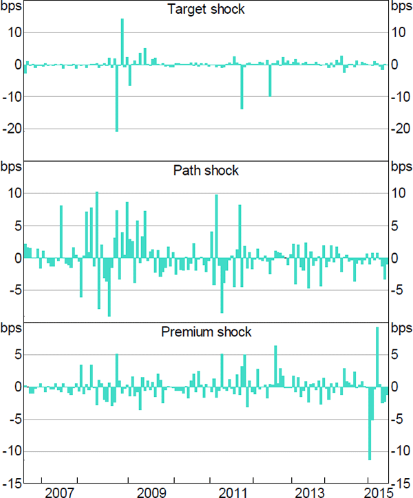
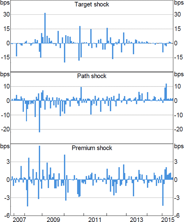
Notes: The figure depicts monetary policy shocks by the European Central Bank, computed based on the repricing of various interest rates on the release of monetary policy news; the top panel shows target shocks as estimated via the change in 1-month OIS rates in a (+/−) 20-minute window around ECB monetary policy announcements; the middle panel shows path shocks as the change in 2-year German government yields orthogonalised against the change in 1-month OIS rates; the bottom panel shows premium shocks as the change in 10-year German government bond yields orthogonalised against the change in 2-year bond yields
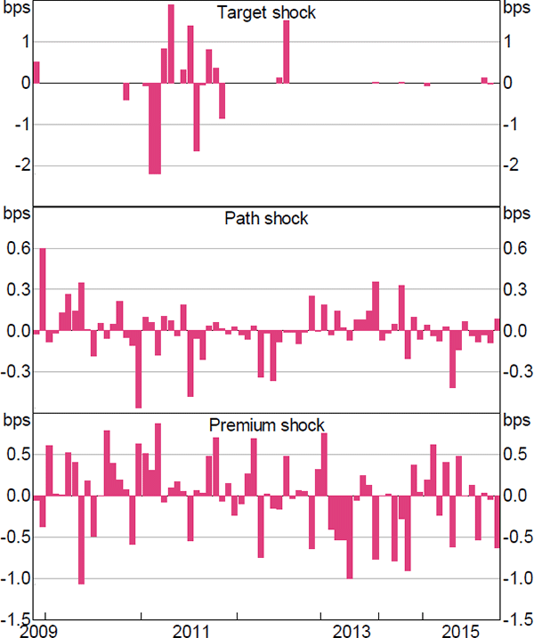
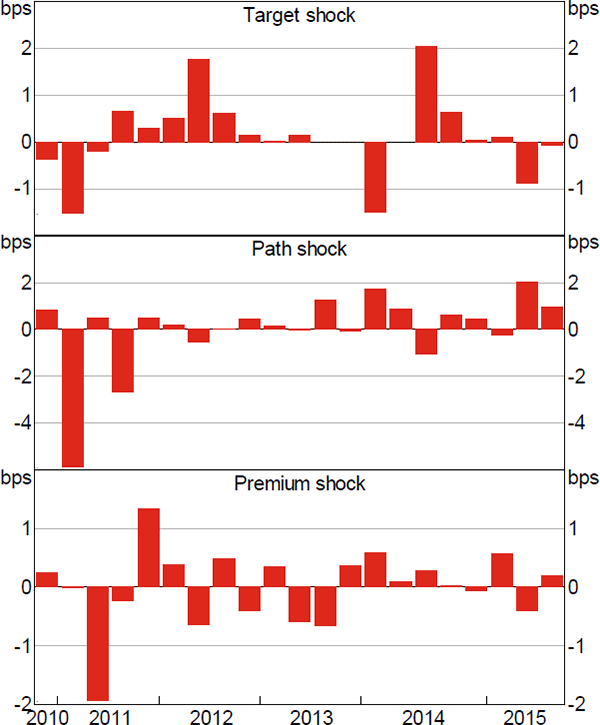
Notes: The figure depicts monetary policy shocks by the Bank of Japan, computed based on the repricing of various interest rates on the release of monetary policy news; the top panel shows target shocks as estimated via the change in 1-month OIS rates in a (+/−) 20-minute window around BoJ monetary policy announcements; the middle panel shows path shocks as the change in 2-year Japanese government yields orthogonalised against the change in 1-month OIS rates; the bottom panel shows premium shocks as the change in 10-year Japanese government bond yields orthogonalised against the change in 2-year bond yields
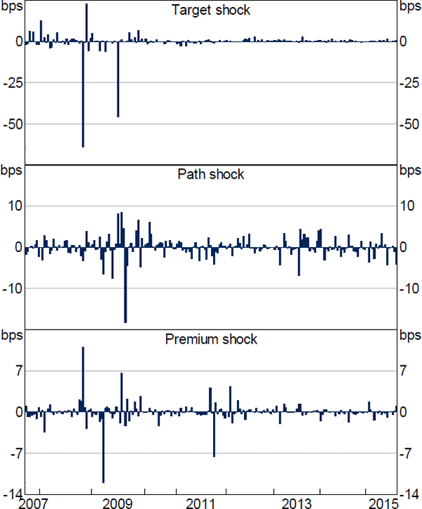
Notes: The figure depicts monetary policy shocks by the Bank of England, computed based on the repricing of various interest rates on the release of monetary policy news; the top panel shows target shocks as estimated via the change in 1-month OIS rates in a (+/−) 20-minute window around BoE monetary policy announcements; the middle panel shows path shocks as the change in 2-year UK government yields orthogonalised against the change in 1-month OIS rates; the bottom panel shows premium shocks as the change in 10-year UK government bond yields orthogonalised against the change in 2-year bond yields
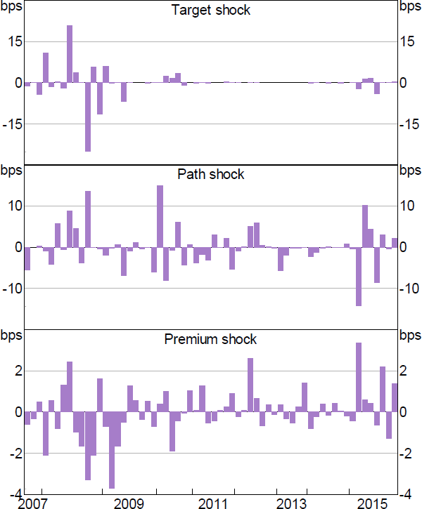
Notes: The figure depicts monetary policy shocks by the Bank of Canada, computed based on the repricing of various interest rates on the release of monetary policy news; the top panel shows target shocks as estimated via the change in 1-month OIS rates in a (+/−) 20-minute window around BoC monetary policy announcements; the middle panel shows path shocks as the change in 2-year Canadian government yields orthogonalised against the change in 1-month OIS rates; the bottom panel shows premium shocks as the change in 10-year Canadian government bond yields orthogonalised against the change in 2-year bond yields
Notes: The figure depicts monetary policy shocks by the Reserve Bank of Australia, computed based on the repricing of various interest rates on the release of monetary policy news; the top panel shows target shocks as estimated via the change in 1-month OIS rates in a (+/−) 20-minute window around RBA monetary policy announcements; the middle panel shows path shocks as the change in 2-year Australian government yields orthogonalised against the change in 1-month OIS rates; the bottom panel shows premium shocks as the change in 10-year Australian government bond yields orthogonalised against the change in 2-year bond yields
Notes: The figure depicts monetary policy shocks by the Swiss National Bank, computed based on the repricing of various interest rates on the release of monetary policy news; the top panel shows target shocks as estimated via the change in 1-month OIS rates in a (+/−) 20-minute window around SNB monetary policy announcements; the middle panel shows path shocks as the change in 2-year Swiss government yields orthogonalised against the change in 1-month OIS rates; the bottom panel shows premium shocks as the change in 10-year Swiss government bond yields orthogonalised against the change in 2-year bond yields
| Target | Path | Premia | R2 (%) | ||
|---|---|---|---|---|---|
| Foreign currency debt | ECB | 0.06 | 0.05 | 0.13 | 2.6 |
| (1.50) | (1.36) | (2.28) | |||
| ECB (excl EA) | 0.00 | 0.12 | 0.13 | 3.6 | |
| (0.04) | (3.57) | (2.39) | |||
| Fed | 0.09 | 0.05 | 0.00 | 5.7 | |
| (2.00) | (1.97) | (0.15) | |||
| Portfolio debt from originator economy | ECB | −0.10 | 0.09 | 0.08 | 2.4 |
| (−1.50) | (1.81) | (0.98) | |||
| ECB (excl EA) | 0.08 | 0.13 | 0.17 | 3.5 | |
| (1.56) | (3.18) | (3.23) | |||
| Fed | 0.04 | 0.02 | 0.10 | 5.0 | |
| (0.75) | (0.56) | (2.68) | |||
| Portfolio equity from originator economy | ECB | 0.00 | 0.16 | 0.08 | 2.4 |
| (0.06) | (3.77) | (1.86) | |||
| ECB (excl EA) | 0.02 | 0.06 | 0.05 | 3.1 | |
| (0.62) | (2.23) | (1.18) | |||
| Fed | 0.03 | 0.00 | 0.12 | 5.0 | |
| (0.43) | (−0.01) | (2.51) | |||
| Loan from originator economy | ECB | −0.09 | 0.09 | −0.02 | 2.3 |
| (−1.94) | (2.34) | (−0.22) | |||
| ECB (excl EA) | −0.03 | 0.09 | 0.10 | 3.2 | |
| (−0.85) | (2.89) | (1.59) | |||
| Fed | 0.00 | −0.02 | 0.02 | 4.8 | |
| (0.10) | (−0.77) | (0.67) | |||
| FDI from originator economy | ECB | −0.02 | 0.06 | 0.03 | 3.5 |
| (−0.61) | (1.95) | (0.63) | |||
| ECB (excl EA) | −0.08 | 0.01 | −0.05 | 9.3 | |
| (−2.51) | (0.44) | (−1.05) | |||
| Fed | 0.02 | 0.00 | 0.02 | 9.1 | |
| (0.47) | (0.07) | (0.89) | |||
| Portfolio debt to originator economy | ECB | 0.07 | 0.14 | 0.16 | 2.7 |
| (1.28) | (3.40) | (2.35) | |||
| ECB (excl EA) | 0.11 | 0.08 | 0.15 | 3.9 | |
| (2.30) | (1.98) | (2.33) | |||
| Fed | 0.02 | −0.04 | 0.01 | 5.1 | |
| (0.41) | (−1.18) | (0.21) | |||
| Portfolio equity to originator economy | ECB | 0.09 | 0.14 | 0.15 | 3.5 |
| (1.90) | (3.43) | (2.61) | |||
| ECB (excl EA) | 0.08 | 0.09 | 0.12 | 6.8 | |
| (2.24) | (2.62) | (2.04) | |||
| Fed | 0.01 | −0.02 | 0.10 | 4.9 | |
| (0.09) | (−0.65) | (2.19) | |||
| Loan to originator economy | ECB | 0.02 | 0.09 | 0.16 | 3.7 |
| (0.33) | (2.50) | (2.05) | |||
| ECB (excl EA) | −0.03 | 0.08 | 0.14 | 3.3 | |
| (−0.93) | (2.51) | (3.03) | |||
| Fed | −0.01 | −0.03 | −0.01 | 8.1 | |
| (−0.36) | (−1.21) | (−0.21) | |||
| FDI to originator economy | ECB | 0.04 | 0.11 | 0.08 | 2.5 |
| (1.20) | (3.74) | (1.73) | |||
| ECB (excl EA) | 0.07 | 0.06 | 0.05 | 3.2 | |
| (2.51) | (2.26) | (1.25) | |||
| Fed | −0.04 | −0.04 | 0.01 | 5.5 | |
| (−1.12) | (−2.06) | (0.53) | |||
| Notes: The table reports the results of panel regressions as given by Equation (2) with various recipient-specific conditional variable Xi,t − 1 measuring bilateral financial openness; the dependent variable is the daily change in 10-year bond yields in our set of 47 recipient economies; as regressors, besides the monetary shocks for the ECB and the Fed, specifications also include the daily change in the US Treasury yield and the VIX as global controls; the reported coefficients correspond to in Equation (2); t-stat from panel-corrected standard errors (PCSE) are given in parentheses; cells coloured red (blue) indicate statistically significant positive (negative) coefficients at a 10 per cent confidence level; financial flows (per cent of GDP) are measured in standard deviations from the mean | |||||
| Target | Path | Premium | R2 (%) | ||
|---|---|---|---|---|---|
| Chinn-Ito index | ECB | −0.09 | 0.10 | 0.08 | 2.7 |
| (−2.01) | (2.64) | (1.25) | |||
| Fed | −0.04 | −0.04 | 0.07 | 5.7 | |
| (−0.54) | (−1.09) | (1.55) | |||
| Debt assets | ECB | −0.02 | 0.08 | 0.14 | 2.5 |
| (−0.47) | (2.67) | (2.77) | |||
| Fed | 0.02 | −0.02 | 0.02 | 5.5 | |
| (0.34) | (−0.80) | (0.72) | |||
| Portfolio assets | ECB | 0.02 | 0.09 | 0.18 | 2.6 |
| (0.44) | (2.28) | (3.42) | |||
| Fed | 0.04 | 0.00 | 0.10 | 5.6 | |
| (0.71) | (−0.14) | (2.52) | |||
| FDI assets | ECB | 0.00 | 0.10 | 0.14 | 2.6 |
| (−0.10) | (3.10) | (3.07) | |||
| Fed | 0.03 | 0.01 | 0.06 | 5.5 | |
| (0.55) | (0.26) | (1.94) | |||
| Financial derivatives | ECB | 0.00 | 0.10 | 0.17 | 2.6 |
| (−0.02) | (2.84) | (3.47) | |||
| Fed | 0.00 | 0.05 | 0.01 | 5.5 | |
| (−0.06) | (1.09) | (0.38) | |||
| Debt liabilities | ECB | −0.06 | 0.10 | 0.14 | 2.6 |
| (−1.33) | (2.64) | (2.08) | |||
| Fed | 0.01 | −0.02 | 0.03 | 5.5 | |
| (0.18) | (−0.64) | (1.04) | |||
| Portfolio liabilities | ECB | 0.00 | 0.07 | 0.10 | 2.5 |
| (−0.06) | (1.86) | (2.31) | |||
| Fed | 0.04 | −0.02 | 0.06 | 5.5 | |
| (0.62) | (−0.72) | (1.75) | |||
| FDI liabilities | ECB | −0.01 | 0.08 | 0.13 | 2.5 |
| (−0.17) | (2.62) | (3.06) | |||
| Fed | 0.03 | 0.02 | 0.05 | 5.5 | |
| (0.77) | (0.64) | (2.06) | |||
| Financial derivative liabilities | ECB | 0.00 | 0.10 | 0.16 | 2.6 |
| (−0.11) | (2.96) | (3.42) | |||
| Fed | −0.01 | 0.05 | 0.01 | 5.5 | |
| (−0.10) | (1.10) | (0.31) | |||
|
Notes: The table reports the results of panel regressions as given by Equation (2) with various recipient-specific conditional variable Xi,t − 1 measuring bilateral financial openness; the dependent variable is the daily change in 10-year bond yields in our set of 47 recipient economies; as regressors, besides the monetary shocks for the ECB and the Fed, specifications also include the daily change in the US Treasury yield and the VIX as global controls; the reported coefficients correspond to in Equation (2); t-stat from PCSE are given in parentheses; cells coloured red (blue) indicate statistically significant positive (negative) coefficients at a 10 per cent confidence level; financial stocks (per cent of GDP) are measured in standard deviations from the mean |
|||||