Research Discussion Paper – RDP 2019-01 A Model of the Australian Housing Market
March 2019
Supplementary Information
Read me file
This ‘read me’ file contains details of the code and data used in RDP 2019-01. Relevant files are contained within ‘rdp-2019-01-supplementary-information.zip’.
Figure data
Publically available plotting data for figures appearing in the RDP can be found in the spreadsheet: rdp-2019-01-graph-data.xls. Data are not available for the ‘Rental yield (matched sample)’ series in Figure 11 due to copyright restrictions.
Running the model
Results were generated using EViews 10 (note, however, that the code was written using EViews 9).
To estimate the model, run the program named ‘_main_program.prg’. This program:
- sets up the EViews workfile and reads in the data,
- defines the values for a number of important strings that are used by the model, and
- runs a succession of sub-programs that estimate the model and put together the graphs/results presented in the paper.
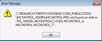
Note: The ‘mcontrol’ add-in is needed for the historical simulations shown in Figures 13 and 14. If the add-in is not installed, you will receive the error message below. See the section ‘Required EViews add-in (mcontrol)’ for more details.
Interpreting the results
After you have successfully run the program, you will have an EViews workfile with a large number of series, graphs, equations, etc.
- Online Appendix D provides a list of the different mnemonics for the variables in the Eviews workfile.
- The graphs shown in the paper are saved using the syntax _gr_02 for Figure 2, _gr_03 for Figure 3, etc.
- Variables with the suffix ‘_b’ show the model’s baseline projections. Variables with other suffixes show projections for alternative scenarios. For example, variables with the suffix ‘_12a’ are used to calculate the responses to a permanent change in interest rates shown in Figure 12 in the paper.
- The EViews model object is named ‘model’. This provides details on all of the equations/identities/ assumptions used by the model.
- The individual OLS equations are also saved in the workfile, with the prefix ‘eq_’. The state-space equations for building approvals have the prefix ‘ss_’.
Directory
Excel files
There are two excel files in the ‘Code_publication’ folder.
- ‘eviews_data.xlsx’ contains all of the data that is initially imported into EViews and used by the model.
- ‘graph_data.xlsx’ contains the data used in the graphs in the paper (except for the matched rental yield in Figure 11 which is available by subscription to CoreLogic). There may be minor differences between this data and that used in the paper arising from data revisions.
Programs
‘_main_program.prg’ provides a brief description of the different sub-programs in this folder, which we have also included below. More detailed comments are provided in each of the sub-programs.
'Data transformations
include 0_data_forward_rates
'Construct forward curve
include 0_data_transformations
'Data transformations and adjustments
'Estimate equations and merge into a model
include 1_housing_approvals_eqns
'Estimate housing approvals equations
include 2_housing_market_eqns
'Estimate equations for housing prices, rents, rental vacancy rate, population
and income
include 3_construction_mapping_eqns
'Estimate housing construction mapping equations (e.g. approvals to
commencements, commencements to work done, etc)
include 4_merge_model_eqns
'Merge the different equations and identities in a model object
'Estimate projections and user-specified model multipliers
include 5_baseline_projections
'Calculate model projections
include 6_alternative_projections
'Calculate responses to the user-specified shock and model projections
'Graph baseline projections and user-specified responses
include 7a_graph_projections
'Put together 9-panel graphs for baseline projections.
include 7b_graph_responses
'Put together 9-panel graphs for responses to user-specified shock.
'Put together graphs shown in the paper (excluding historical simulations)
include 8_graph12_cash
'Graph 12 - Responses to percentage point reduction in interest rates
include 8_graph15_approvals
'Graph 15 - Responses to dwelling approvals
include 8_graph16_price_expectations
'Graph 16 - Responses to housing price appreciation expectations
include 8_other_graphs
'Other graphs used in the paper
'Historical simulations
include 9_historical_simulations
'Estimate historical simulations and put together graphs
‘Responses’ folder
This folder contains the estimated responses to changes in a number of important variables in our model. These variables are:
– Total building approvals (chain volume measure) (batotalvol)
– Cash rate (cash)
– Real dwelling prices (rdp)
– Real household disposable income (rinc)
– Real CPI rents (rent_cpi)
– Adult population (wap)
The graphs include responses to permanent changes in these variables (in the sub-folder ‘perm’), as well as 4-quarter changes (‘temp’) and 1-quarter pings (‘ping’).
‘mcontrol_addin’ folder
This folder contains the version of the ‘mcontrol’ add-in used in our paper. See below.
Required EViews add-in (mcontrol)
The ‘mcontrol’ add-in is needed for the historical simulations in Saunders and Tulip (2019). These simulations are run from ‘9_historical_simulations.prg’.
There are a couple of ways to install this add-in.
- The simplest method is to open ‘_main_program.prg’, uncomment the line of code ‘exec %mcontrol_addin’ (line 21), and run the program. This will install the add-in from the folder ‘mcontrol_addin’. A benefit of this method is that it will install the version of the add-in used in the paper, so the results will be replicable. A disadvantage is that the add-in might need to be re-installed if the name or location of the folder is changed after the initial install. See below for more details.
- You can also install the add-in from the EViews website. Go to the EViews add-in website (http://www.eviews.com/Addins/addins.shtml), find and click on the mcontrol hyperlink, and follow the prompts. This will install the latest version of the add-in, so the results may not match the historical simulations in Saunders and Tulip (2019) if the add-in has been updated.
Changing the file path for mcontrol add-in
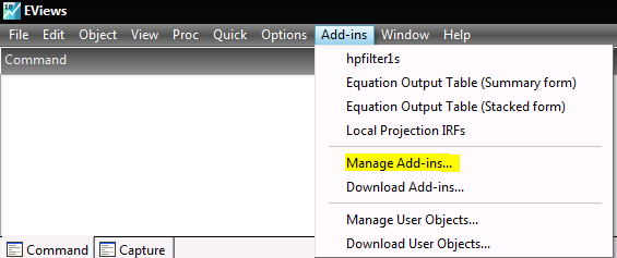
You might receive an error message if the name or location of the folder is changed after the initial installation of the mcontrol add-in. If this happens, you will need to update the location of the mcontrol add-in so that EViews knows where to find it. To do this:
– Open EViews.
– Go to the ‘Add-ins’ drop down menu and click on ‘Manage Add-ins’ (see below).
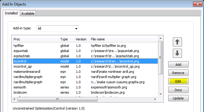
– Highlight the mcontrol add-in and click the ‘Edit’ button. (Note: There is also an add-in named ‘mcontrol_qp’, which is not used by the housing model).
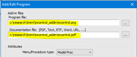
– Change the path for the add-in and documentation to the new location.
Including state-space equations in EViews model objects
We estimate the different building approval equations with time-varying intercepts. Unfortunately, you cannot include state-space equations in EViews model objects (i.e. we can’t directly include these equations in the model).
To get around this issue, we have:
- saved the 2-sided estimates of the time-varying intercepts from the state-space equations,
- included these time-varying intercepts in OLS versions of the equations (with the coefficients on the intercepts restricted to equal 1), and
- included these OLS equations in the model.
These OLS equations have the same coefficients as the state-space equations, so will produce the same projections and model multipliers. The standard errors for the OLS versions of the equations will be wrong though.
Bibliography material
Fox R and P Tulip (2014), ‘Is Housing Overvalued?’, RBA Research Discussion Paper No 2014-06.
- Supplementary information