RDP 2018-12: Where's the Money? An Investigation into the Whereabouts and Uses of Australian Banknotes 4. Cash Used in Legitimate Transactions
December 2018
- Download the Paper 1,608KB
We now turn to estimating the outstanding stock of banknotes used to facilitate legitimate transactions in Australia. We employ five different methods based on a ground-up count, the life and processing frequencies of different denominations, the velocity of banknotes in circulation, and the seasonality of outstanding banknotes.
4.1 The Counting Method
4.1.1 Method
The first approach is a direct one. We estimate the transactional stock of cash from the ground up. This means estimating the stock of cash held in various physical locations that we consider to be part of the transactional stock, and aggregating them to form an economy-wide estimate. This calculation by necessity relies on a number of assumptions, and will miss any cash held in locations not directly considered. Despite these drawbacks the approach is useful as it provides a broad sense-check on other estimates arrived at through more abstract means, and also offers a tangible basis to think about the transactional stock of cash.
The locations we consider to be part of the transactional stock are listed in Table 1. We use two approaches to estimate the stock of cash held in each of these locations:
- Estimating the number of particular locations (e.g. the number of tills) and multiplying this by an estimated average amount held per location. Where appropriate, these estimates are deflated/inflated by other series (e.g. population, inflation or a measure of economic activity).
- Converting flow data to a stock by making assumptions about the velocity of cash through a particular location.
| Location | Description |
|---|---|
| Wallets | Cash held by consumers on their person. |
| Financial institution holdings |
Cash held by financial institutions including in ATMs, bank branches and cash depots, as well as cash in transit. |
| Tills and self-service check-outs | Cash held in tills and cash-accepting self-service check-outs at the start of business. This is the minimum stock of banknotes that is held at all times. It does not include cash held due to an increase in stocks from consumers' cash expenditure. |
| Unbanked business takings | Cash held by businesses due to consumers' cash expenditure that has not been banked. |
| Gaming machines | Cash held in gaming machines (e.g. poker machines). |
| Tourists | Cash held by tourists in Australia or about to enter Australia. This includes cash sourced overseas prior to entering Australia and cash sourced domestically after entering Australia. Cash held by overseas foreign exchange businesses that service tourists about to enter Australia is also included here. |
A more detailed explanation of the specific methodology used to estimate the stock of cash held in each location can be found in Appendix A.
4.1.2 Results
This method suggests that the transactional stock of cash has risen from around $9 billion at the end of 2002 to around $13 billion as at June 2018 (Figure 5). This corresponds to an annualised growth rate of around 2 per cent, although growth is estimated to have been slightly slower over the past five years.
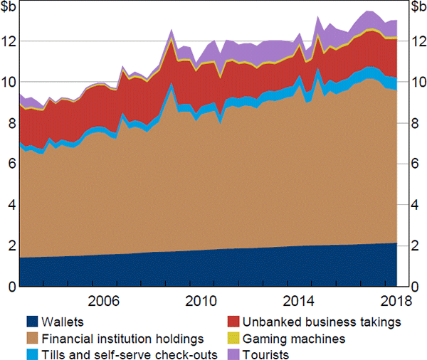
Sources: ABS; Australian Payments Network; Authors' calculations, based on data from Colmar Brunton, Ipsos, RBA and Roy Morgan Research; Queensland Treasury; Tourism Research Australia; Wesfarmers; Woolworths Group
In dollar terms, financial institution holdings drove most of the increase in the total transactional stock, although most components have grown since 2002. In fact, the only component that is estimated not to have grown since 2002 is unbanked business takings. This follows from relatively stable cash expenditure, as growth in total nominal spending has been offset by changes in consumers' payment preferences.
While the transactional stock estimated using this method has increased since 2002, it has not kept pace with the increase in total outstanding banknotes, which has grown at around 6 per cent per annum over this period. As a result, the transactional stock's share in total outstanding banknotes is estimated to have fallen from 30 per cent to a little under 20 per cent according to this method.
4.2 The Banknote Life Method
4.2.1 Method
Banknotes reach the end of their lives (become ‘unfit’) for two main reasons: excessive inkwear, which will tend to increase in a relatively linear fashion with banknote use; and mechanical defects such as tears, which can be thought of as random events that can occur at any stage, but whose cumulative probability of having occurred also increases with use. We measure banknote life as the average number of banknotes outstanding over a given period, divided by the number of banknotes that have been deemed unfit over the same period, and choose a five-year period to average over in order to reduce undue volatility.[6] When performing this calculation we also adjust the number of outstanding banknotes for our estimate of lost banknotes, using the midpoint of our 5–10 per cent loss range.
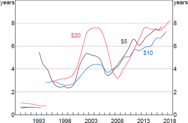
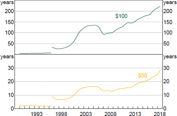
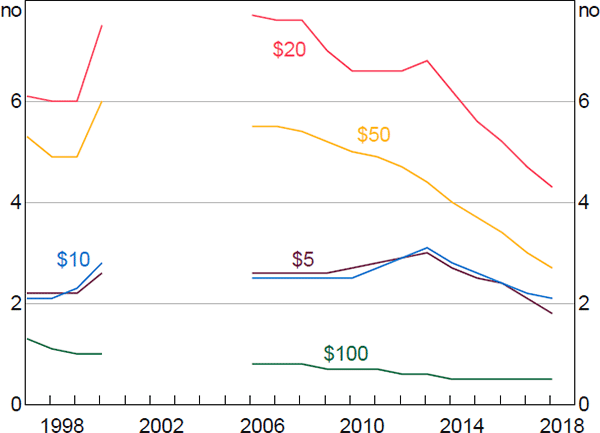
Figures 6 and 7 show estimated banknote life, from which one can observe that: polymer banknotes have a much longer life span than paper banknotes; low-denomination banknotes ($5, $10 and $20) have broadly similar banknote life; and high-denomination banknotes ($50 and $100) have a longer life span than low-denomination banknotes. Further, one can see that the life span of all banknotes has increased in recent years, which could reflect improvements in banknote handling, a decline in the velocity of transactional cash, and/or the after-effects of previous banknote cleansing programs, which replaced old banknotes with new ones, reducing measured banknote life at the time and increasing the quality (and remaining life) of the cleansed outstanding stock.
Given that all denominations of banknotes are initially of similar quality, the speed at which certain denominations become unfit is closely related to the frequency with which they are handled. Since banknotes are most commonly handled when used as a means of payment, banknotes used in transactions should have a shorter life span than banknotes not used in transactions.
Notes: Initial data are paper, later data are polymer; excludes periods when issuance of new series banknotes materially affected data; banknote distribution arrangements were changed in the early 2000s, resulting in a large stock of banknotes entering circulation and temporarily boosting estimated life
Sources: Authors' calculations; RBA
For our estimates, we assume that low-denomination banknotes are used only for transactional purposes. Although this may not be exactly true, it is likely to be a close approximation of reality as the low value of these banknotes relative to the $50 and $100 make them an inefficient store of value. That they all have similar life spans further supports the idea that they are used for similar purposes (Figure 6). For example, if the $20 was hoarded significantly more than the $10, we would expect that to manifest in a longer life for $20 banknotes, whereas this is not the case. Nonetheless, we note that if a large volume of low-denomination banknotes are actually used for non-transactional purposes, our estimates of the transactional stock will be upwardly biased.
Moreover, we assume that all banknotes used for transactional purposes are handled an equal number of times and with equal care. This assumption is arguably more tenuous: high-denomination banknotes used for transactions may be treated with more care than low-denomination banknotes and, further, may be handled less frequently because they are less likely to be given as change (e.g. the $100 will never be given as change). To the extent that this assumption does not hold, our estimates of the transactional stock will be downwardly biased.
Working the other way, even if transactional high-denomination banknotes are used less frequently for payments than low-denomination banknotes, high-denomination banknotes are more likely to pass through ATMs and other banknote processing machines, and so be quality-screened and ‘handled’ in that way; if the process of being stocked in and withdrawn from ATMs is particularly wearing, and/or the more frequent quality-screening allows these banknotes to be withdrawn from circulation earlier than lower denomination banknotes that are quality-screened less often, this will upwardly bias our transactional stock estimates.
If the net effect of all these potential issues had large effects on banknote life, we might expect this to show up in the $20, which is both less likely to be given as change than the $5 and $10, and is far more likely to be quality-screened and passed through ATMs. The fact that the $20 has a very similar life to the $5 and $10 therefore provides some comfort these issues are not materially affecting our results.
Given these assumptions, any ‘excess life’ of high-denomination banknotes, relative to low-denomination banknotes, can be attributed to the non-transactional uses that they facilitate (e.g. store of value), and so can be used to estimate the split between transactional and non-transactional cash. In particular, assuming that transactional high-denomination banknotes have the same life span as lower denomination banknotes (all of which are assumed to be used for transactions), the excess life of $50 and $100 banknotes, relative to the average life of the lower denominations, divided by the average life of the higher denominations, gives the estimated share of non-transactional high-denomination banknotes. Intuitively, imagine that one in four $50 banknotes is used for transactions and three in four are hoarded. The hoarded banknotes will never become unfit as they lie untouched. The transactional $50 banknotes should become unfit at the same rate as the lower denominations, assuming that they are handled in a similar fashion. Accordingly, the ratio of total to unfit banknotes over a given period (i.e. ‘banknote life’) should be four times higher for $50 banknotes relative to the lower denominations, and the above calculation will give a result of three-quarters (see Appendix B for the mathematics). Boeschoten (1992) uses a similar method to estimate hoarding in the Netherlands, while Bartzsch, Rösl and Seitz (2011) employ the method using the differing average ages of German and French banknotes, rather than between denominations, to estimate the transactional share of German banknotes.
To ensure that the issuance of new series NGB banknotes has no effect on our estimates, we exclude denominations from our calculations from the date of NGB issuance. We also exclude estimates for periods when the issuance of the polymer banknotes materially affected the data (the mid 1990s), but include data around the early 2000s when a change to banknote distribution arrangements artificially boosted estimated banknote life (as all denominations were affected, the net result on our transactional stock estimates is small; see Figure 8); we make no attempt to adjust for earlier banknote cleansing programs, with the five-year averaging of banknote life that we use designed to mitigate various idiosyncratic shocks to individual banknote life series.
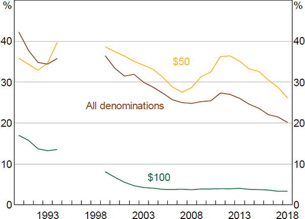
Notes: Initial data are paper, later data are polymer; excludes periods when issuance of new series banknotes materially affected data
Sources: Authors' calculations; RBA
4.2.2 Results
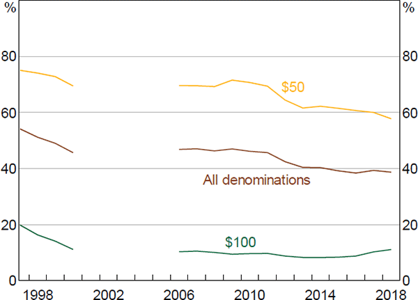
Over the past three decades we estimate that: the share of $100 banknotes used for transactions has fallen from around 20 per cent to just 3 per cent; the share of $50 banknotes used for transactions has fallen from around 35 per cent to 25 per cent; and the transactional share by value of all banknotes has fallen from around 45 per cent to around 20 per cent (Figure 8). Excluding the $100 banknote, which is overwhelmingly used for non-transactional purposes, we estimate that the transactional share of the lower four denominations is around 35 per cent. Given that this method makes no distinction between cash used for legitimate and illegitimate purposes, subtracting an estimated 5 per cent of cash used for shadow economy transactions (see Section 5.4) suggests that the overall transactional share, restricted to legal transactions, is around 15 per cent of outstanding banknotes.
If we relax the assumption that all transactional banknotes should have equal life and instead assume that transactional $50 and $100 banknotes last twice as long as the lower denominations, say, perhaps due to more careful handling for example, then the implied transactional share of $50 and $100 banknotes is double that given in Figure 8, and the overall transactional share of outstanding banknotes falls from 65 per cent three decades ago to 35 per cent today, or around 30 per cent after subtracting cash used in shadow economy transactions.
As noted, the above figures assume that around 7½ per cent of banknotes recorded as outstanding have actually been lost, and adjust for this. If we do not adjust for lost banknotes, the transactional share estimates above are boosted by around 2 percentage points.
4.3 The Banknote Processing Frequency Method
One can apply the same idea used in Section 4.2 to data on the frequency with which different banknote denominations are processed by cash depots. In particular, cash depots process and fitness-sort banknotes lodged by commercial banks and large retailers, and importantly do not process any banknotes that are hoarded or otherwise not part of the transactional stock of cash. Thus, broadly speaking, only the transactional stock of banknotes passes through cash depots, and the rate at which banknotes pass through depots is an indication of transactional cash use.
Figure 9 shows the average number of times each banknote denomination passes through a cash depot per year, and a few features are worth observing. First, in recent years there has been a general decline in the banknote processing frequencies of all denominations. This is consistent with a fall in the velocity of cash and/or consumers substituting away from cash as a means of payment, both of which result in banknotes passing through depots less frequently. Second, we see that the $50 and $100 banknotes pass through depots less frequently than $20 banknotes, which is indicative of non-transactional demand for these denominations given that, once spent, they are very likely to be banked (retailers don't keep $100 banknotes to use as change). Conversely, the low processing frequency for the $5 and $10 banknotes is most likely due to their use as change – that is, they cycle between consumers and retailers many times before being returned to a cash depot for processing.
Notes: Excludes periods when changes in banknote distribution arrangements materially affected the data; data either side of the break are not directly comparable
Sources: Authors' calculations; RBA
Given these observations, we make two assumptions:
- the non-transactional stock consists only of $50 and $100 banknotes;
- the processing frequency of the transactional stock of $50 and $100 banknotes is equal to the processing frequency of the $20 banknote.
These assumptions imply that non-transactional demand is the reason that the processing frequency of $50 and $100 banknotes is less than for $20 banknotes, and allow us to estimate the extent of hoarding of the higher denominations. As discussed in Section 4.2, the first assumption, while not entirely true, is likely to be broadly accurate. The second assumption is somewhat more tenuous, however, as the true processing frequency of the transactional stock of $50 and $100 banknotes is likely to be higher than for the $20 as almost all $50 and $100 banknotes received by retailers are likely to be banked, whereas some $20 banknotes will be given as change. This will result in an upwardly-biased transactional share estimate.
The results of this method suggest that the transactional stock has fallen from around 55 per cent of total outstanding banknotes in the late 1990s to around 40 per cent now, or 35 per cent after subtracting cash used in shadow economy transactions (Figure 10). As above, these figures adjust for estimated lost banknotes; removing this adjustment boosts the estimated transactional share by around 3 percentage points.
Note: Excludes periods when changes in banknote distribution arrangements materially affected the data
Sources: Authors' calculations; RBA
4.4 The Velocity Method
An important determinant of the stock of cash needed to facilitate transactional demand is the flow of payments made using cash. However, the flow of cash payments does not, on its own, tell you about the stock of cash used to facilitate transactions, as one banknote can be used in multiple transactions over a period. To connect the flow of cash payments with the transactional stock, we need to have an understanding of the velocity of cash: the average number of times the transactional stock is used in a given period. For example, if the flow of total cash payments in a month was $20 billion, and the transactional stock of cash was $10 billion, the entire stock must have turned over twice in the month: velocity, in units per months, would be 2. This concept is summarised in the following equation:
We now turn to estimating flow of cash payments and the velocity of transactional cash in order to estimate the value of the transactional stock of cash.
4.4.1 The value of cash payments
Long-term determinants of cash payments include consumer payment preferences, accessibility of alternative payment methods, and macroeconomic factors such as nominal consumer spending and interest rates. Unlike card payments, however, the value of cash payments is not observed directly and so must be estimated. To do so we distinguish between payments made using cash sourced within Australia and cash sourced overseas. We estimate the value of cash payments made with cash sourced in Australia by scaling card payment data collected by the Reserve Bank with the cash-to-card payment ratio from the CPS.[7] To approximate the value of cash payments made with cash sourced from overseas, we subtract the value of card payments and ATM withdrawals made with international cards from estimated total tourist spending obtained from Tourism Research Australia, and also adjust for estimates of tourists' domestically sourced income.[8]
Applying this approach, Figure 11 shows estimated total cash payments increasing over the past four years, after declining by approximately 40 per cent between 2007 and 2013. This stabilisation and rebound is a function of consistent growth in total payments (due to factors such as population and nominal income growth), combined with the cash-to-card ratio by value recorded in the 2016 CPS being little changed from 2013 (despite the ratio by number falling substantially). The earlier sharp fall is driven by a steep decline in the cash-to-card ratio between 2010 and 2013.[9]
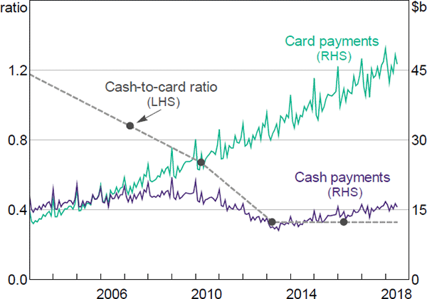
Notes: Card payments includes payments made by businesses using debit cards; dashed line indicates points that have been interpolated or extrapolated; dots indicate direct estimates from the CPS
Sources: Authors' calculations, based on data from Colmar Brunton, Ipsos, RBA and Roy Morgan Research; Tourism Research Australia
4.4.2 The velocity of transactional cash
To estimate the velocity of transactional cash we map out the cash cycle: banknotes start at a cash depot, are transported to an ATM or bank branch, pass to a consumer's wallet or purse, get spent at a business, and then get returned to a bank and/or cash depot. Summing up time-varying estimates of how long it takes cash to pass through each point in the cycle will give an estimate of how long it takes for the transactional stock to turn over. Dividing the number of days in a month by this will give us a monthly estimate of velocity. We work with a generic dollar or purchasing power, rather than trying to estimate velocities for individual banknote denominations.
The general approach we follow for estimating the number of days it takes for cash to pass through a point in the cash cycle is: if there is continual inflow and outflow of cash, we divide the average value of the stock of cash by the daily outflow of cash (this will be exactly correct if cash is first-in-first-out and the daily stock and outflow is constant, and approximately correct otherwise); or, if there is continual outflow of cash but periodic inflow, we take half the average time between inflows. Importantly, many businesses, individuals and ATM operators keep a buffer stock of cash; instead of letting their cash holdings run to zero, they fill up their wallet or ATM when their cash gets below a certain threshold. We account for this by factoring in buffer thresholds (denoted as r) to our estimates. The buffer threshold is expressed as a percentage of the average full amount, while the sizes of the buffer stocks that we set are informed by liaison and our own judgement (see Appendix C for further details). In detail, the average time spent in each location is estimated as follows:
- cash depot: (total value in depot)/(daily depot outflow);
- wallet: ((1 + 2r) × (days in month) ÷ (average number of cash withdrawals per person per month)) ÷ 2; we divide by 2 to get an average time rather than the maximum time that a banknote stays in someone's wallet;
- ATM: ((1+2r) × (days in month) ÷ (average number of ATM refills per month)) ÷ 2; the average number of ATM refills per month is estimated using the total value of ATM withdrawals per month, the total number of ATMs, and the effective capacity of the average ATM;
- cash register or till: (1+2r) × (1 day estimated time spent in till).
Due to a lack of data we assume that cash flows through commercial bank branches take a similar amount of time as flows through ATMs, and deviations from the assumption will bias our results. In addition, we add in approximations of the time cash spends in transit between various holding points (e.g. from a cash depot to an ATM, or from when cash is initially put into a retailer's safe to when it is subsequently deposited at a bank branch). We refer to this as the number of days cash spends in transit. Finally, to estimate the velocity of overseas-sourced cash, we multiply the velocity of domestically sourced cash by a scaling factor.
Given the inherent uncertainty involved in estimating the buffer stocks, the additional time taken for overseas-sourced cash to circulate, and the time banknotes spend in transit, we present three different scenarios. They are summarised in Table 2.
| High velocity | Medium velocity | Low velocity | |
|---|---|---|---|
| Wallet buffer | 5 per cent of average withdrawal | 20 per cent of average withdrawal | 35 per cent of average withdrawal |
| ATM buffer | 5 per cent of capacity | 15 per cent of capacity | 25 per cent of capacity |
| Till buffer(a) | $300 | $500 | $700 |
| Overseas scaling factor | 2 times slower than domestic velocity | 4 times slower than domestic velocity | 6 times slower than domestic velocity |
| Transit time | 3 working days | 5 working days | 7 working days |
| Note: (a) The buffer stock held in tills for the period studied is CPI-adjusted to be equivalent to the listed value in 2017 | |||
4.4.3 Results
Our results suggest that the velocity of transactional cash has declined over the past decade (Figure 12). This is consistent with ATM data showing declining withdrawals and the findings of Flannigan and Staib (2017). Because of rising cash payments and declining velocity, we estimate the transactional stock of cash to be gradually increasing over recent years and in the range of $15–25 billion currently. These results suggest that transactional cash accounts for around 20 to 30 per cent of total outstanding banknotes (Figure 13).[10]
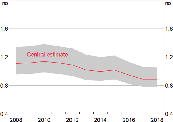
Notes: Domestically sourced cash; overseas velocity is obtained by dividing the estimate by the scaling factor; shaded area denotes the range of velocity assumptions
Sources: Authors' calculations, based on data from Colmar Brunton, Ipsos, RBA and Roy Morgan Research; Tourism Research Australia
Note: Shaded area denotes the range of velocity assumptions
Sources: Authors' calculations, based on data from Colmar Brunton, Ipsos, RBA and Roy Morgan Research; Tourism Research Australia
4.5 The Seasonality Method
Another way to estimate the share of banknotes used regularly in transactions is to study the seasonality of banknote demand.[11] The logic works as follows: demand for cash displays predictable seasonality, with a seasonal peak around Christmas and a seasonal trough in the winter months. This seasonality resembles the seasonality present in consumer spending, which suggests that it is driven by seasonality in transactional cash demand. On the other hand, non-transactional cash demand (e.g. hoarding for store of value or numismatic purposes) is unlikely to contain significant seasonality. As a result, if most cash is transactional, then the seasonality of cash demand should closely match the seasonality of consumer spending; conversely, if the non-transactional stock dominates, then the seasonality of cash demand will be dampened relative to that seen in consumer spending. Thus the magnitude of the seasonality present in cash demand, when compared with the seasonality of consumer spending, is an indication of the share of cash used for transactional purposes.
4.5.1 Method
We begin by considering banknote demand as a simplified multiplicative seasonal model consisting of two terms: a trend component Tt, and a seasonal component St. We can then express the seasonal factors of banknote demand for any period as a linear combination of the seasonality of the transactional stock and the seasonality of the non-transactional stock. Suppressing the subscript t for convenience, we have:
where α is the transactional share of banknotes. We then assume the non-transactional stock of cash displays no seasonal behavior (i.e. SNon-trans = 1).[12] This allows us to solve for α:
While STot is easily computable, STrans is unknown and difficult to estimate without prior knowledge of the size of the transactional stock or a reference variable. To overcome this and as noted earlier, we use the fact that the flow of cash payments and the transactional stock are related via the following equation:
Dividing both sides by velocity and writing each term as its trend and seasonal component gives us the following expression for the transactional stock:
Focusing only on the seasonal components gives:
Therefore, we can model the seasonality of the transactional stock by estimating the seasonality of cash payments and the seasonality of velocity, both of which can be approximated. To do this we explore various variables and compare the results from each. For each variable, we take the difference between the 12-month seasonal peak and seasonal trough as an estimate of seasonality (we refer to this as the seasonal amplitude and take results from June in each year).
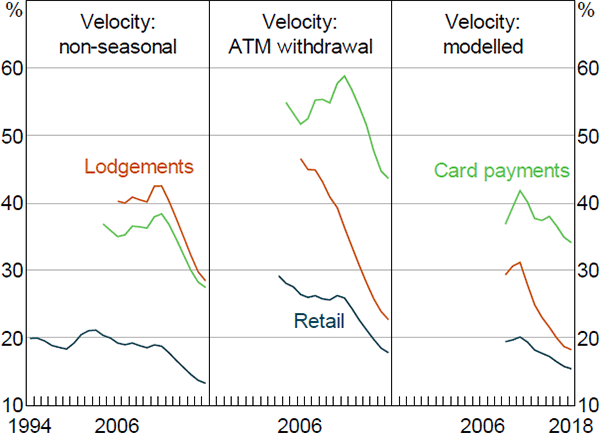
We use the seasonality present in the following variables to approximate the seasonality of cash payments:
The seasonality present in each of these variables is driven by seasonality in spending, which should approximate the seasonality present in cash payments. For retail sales and card payments to be good proxies, however, it is necessary that the substitution rate between cash and non-cash means of payment is non-seasonal; excluding banknote lodgements themselves, which we use directly, there are no good data on this, but there are reasons to believe that it might not be the case. For example, if consumers are relatively more likely to purchase Christmas-related items on credit, the seasonal peak in retail sales will be higher than the true peak in transactional cash demand, and the estimated transactional share of outstanding banknotes will be underestimated. Conversely, if cards (but not cash) are used for types of payments without a strong seasonal pattern (utility bills or school fees, for example), the seasonal pattern of card payments will tend to be dampened relative to the true seasonal pattern of cash spending. Banknote lodgements, on the other hand, which measure cash flowing into cash depots, are a direct measure of cash spending, and so should not suffer from the above issues. However, there are small timing issues with lodgements data. For instance, it is common for seasonal peaks in lodgements to be split across December and January even though cash payments probably peak in December. Using the annual seasonal amplitude in our calculations offsets some of these effects.
To approximate the seasonality of velocity we use three different approaches. First, we assume that velocity is non-seasonal (i.e. SVelocity = 1). This is unlikely to be true in reality. Banknotes probably circulate faster during seasonal peaks in spending and slower during seasonal troughs. However, velocity is intrinsically harder to measure than cash payments, and by including this method we hope to eliminate one potential source of noise from the data while still identifying broad trends. This is particularly relevant if there has been little change in the seasonality of velocity over the period studied. In this case, our levels may be wrong but our trends will be broadly accurate. Second, we use the number of ATM withdrawals per person per month to proxy velocity. We do this as the frequency with which consumers withdraw cash is likely to be correlated with the frequency with which cash more broadly circulates; for example, faster velocity should correspond with more cash top-ups. Finally, we use our estimate of velocity from Section 4.4.
4.5.2 Results
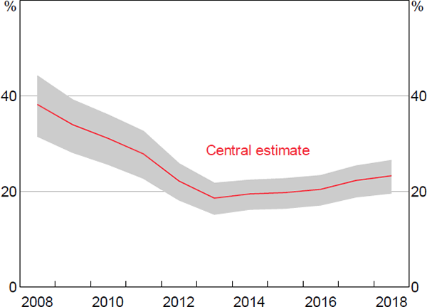
Our estimates using the three proxies for cash spending and the three velocity assumptions are shown in Figure 14. Although there is wide variation, with the latest transaction share estimates ranging from 13 to 44 per cent, a few points stand out:
- all estimates show a substantial decline in the transactional share of cash over recent years, of the order of 10–20 percentage points;
- using retail sales as a proxy for cash payments results in much lower estimates of the transactional stock than the other two variables, which in a mechanical sense is driven by the extreme seasonality of the retail sales variable; and
- for most velocity assumptions, using card payments as a proxy for cash spending tends to produce the highest transactional share estimates, and using retail sales tends to produce the lowest estimates, perhaps for the reasons discussed above.
Sources: ABS; Authors' calculations, based on data from Colmar Brunton, Ipsos, RBA and Roy Morgan Research; Tourism Research Australia
4.5.3 Assessment
The theory and intuition behind the seasonality method is convincing as it describes a simple way to estimate the transactional stock, and so there are good reasons to expect reliable estimates using the above methods. That our results are broadly consistent supports this: all series provide evidence of a material decline in the transactional share over the past decade. Conversely, while the theory is compelling, in practice our results contain considerable variation. In 2018, our estimates of the transactional share range from 13 to 44 per cent of outstanding banknotes: a difference equating to approximately $20 billion. These differences are largely due to three factors: first, for the reasons discussed earlier, retail sales and card payments are imprecise proxies for cash spending. We believe the retail sales approach underestimates the transactional share, while the card payments method likely overestimates the transactional share. Second, modelling the seasonality of velocity by a constant is probably too simplistic, while using the seasonality in ATM withdrawals is better but still not perfect. Both of these approaches at least partly ignore the interplay between velocity and the size of the outstanding transactional stock of cash. For example, while ATM withdrawals increase in December (speeding up velocity), so does the size of cash stocks at cash depots (slowing down the rate at which cash passes through depots). The net effect on velocity depends on the relative size of each. Finally, all of our methods are sensitive to small changes in the seasonality of the data, some of which could be due to the timing differences discussed earlier and not actual changes in the transactional share. This is likely to have the greatest impact when we use our estimate of velocity from Section 4.4 because it draws on many different data sources.
Overall, we believe that banknote lodgements provide the most robust estimate of the flow of cash spending. Regarding velocity, we are cautious to put too much weight on one method, and so use the range of transactional shares suggested by different velocity assumptions. This suggests that the transactional share has declined from 30 to 45 per cent of outstanding banknotes in 2009 to roughly 20 to 30 per cent currently, or 15 to 25 per cent after subtracting cash used in shadow economy transaction. Figure 15 converts these shares to dollar values. We see that only the non-seasonal velocity assumption results in a transactional stock that has grown over the past decade, with the other assumptions implying little to no change.
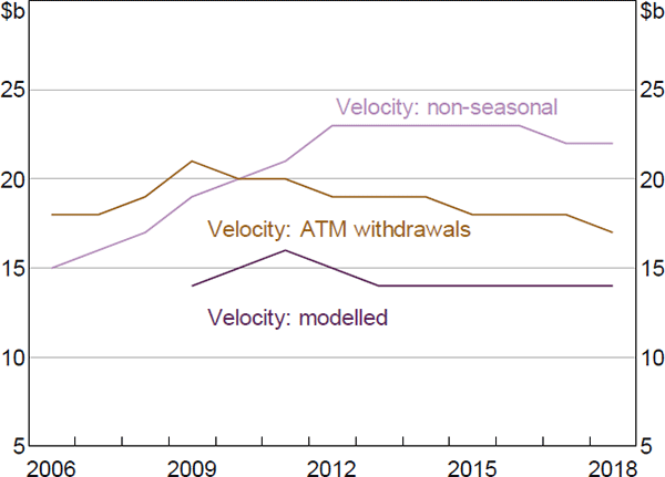
Sources: Authors' calculations; RBA
4.6 Overall Assessment
Overall, the methods employed in Sections 4.1 to 4.5 suggest that somewhere between 15 and 35 per cent of outstanding banknotes are used to facilitate legitimate transactions within Australia. Although each estimation method is imperfect, we take comfort from the fact that a number of very different methods yield broadly similar results. All methods also suggest a decline in the transactional share of total outstanding banknotes of the order of roughly 1–1½ percentage points per year.
Our transactional share estimates are broadly in line with comparable international studies. For example, Fish and Whymark (2015) use a direct counting method similar to that in Section 4.1 to estimate that 21–27 per cent of UK banknotes were used for transactional purposes in 2014, having fallen from 34 to 45 per cent in 2000. Similarly, Gresvik and Kaloudis (2001) estimate via a combination of the direct counting and velocity methods that around 32 per cent of cash holdings in Norway could be explained by transactional use in 2000, while Humphrey, Kaloudis and Øwre (2004) similarly estimate that 37 per cent of cash in Norway could be explained by legal non-hoarding uses (with the residual 63 per cent put down to hoarding and shadow economy activities). For Sweden, Guibourg and Segendorf (2007) estimate that transactional demand for cash explains around 35 per cent of outstanding Swedish banknotes over the period 2000–04, while Lalouette and Esselink (2018) use a processing frequency method to estimate that around one-quarter of euro banknotes are used for transactional purposes within the euro area.[15]
A number of studies use econometric models to indirectly estimate the flow or stock of transactional cash demand. For example, Snellman, Vesala and Humphrey (2001) regress growth in card payments on growth in outstanding currency and growth in GDP, and then use the estimated coefficients to back-out the implied flow demand for transactional cash, controlling for the number of ATM and EFTPOS terminals per person. Seitz (2007) postulates that the stock of transactional cash balances (plus overnight deposits) determines inflation, and estimates the share of cash used for transactions as that which leads to the best-fitting inflation equation. We do not follow these approaches as the assumptions needed to generate results seem unrealistic (in the two examples given, that changing preferences between cash and electronic payment methods over time can be captured by the number of ATM and EFTPOS terminals, and that physical banknote holdings are a major determinant of inflation, respectively), while a more robust method to estimate the flow of transactional cash demand is open to us as discussed in Section 4.4.
Footnotes
This ‘steady-state method’ is described in Rush (2015) and is the standard measure that most countries use to measure banknote life, although it is typically estimated over a one-year period to abstract from seasonal fluctuations. Note that banknote life can be distorted by the issuance of new banknotes and ‘cleansing programs’, which seek to remove large volumes of banknotes from circulation to improve banknote quality. [6]
Respondents to the CPS record all payments made over a week and the method with which each payment was made, allowing us to estimate the ratio of cash to card payments. We interpolate this ratio between survey years and extrapolate the 2013–16 trend for 2017 and 2018. If we instead use ATM withdrawals as a proxy for cash spending we obtain similar results. [7]
Here we project tourist spending forward for the first six months of 2018 to fill in missing data; as this is only a small component of total cash spending, any errors are unlikely to have a material impact. [8]
The 2013 cash-to-card ratio appears to be somewhat of an anomaly, and from a visual inspection appears ‘too low’ when compared with the ratio in 2010 and 2016; if one adjusted the ratio up in line with the pattern displayed by the other three readings, one would see a more gentle but sustained fall in estimated cash spending over the past decade. The 2019 CPS should shed more light on the evolution of consumer payment preferences. [9]
These estimates are unlikely to include cash used in shadow economy transactions as they flow from cash spending as estimated by the cash-to-card ratio from the CPS multiplied by card spending, neither of which are likely to contain shadow economy transactions. [10]
This method was first suggested by Sumner (1990), while Bartzsch et al (2011) and Judson (2012) use a similar approach to estimate the share of currency held offshore. We use X-13ARIMA-SEATS in R to seasonally adjust. [11]
Non-transactional demand is probably dominated by hoarding for store-of-value purposes. The flow of banknotes into hoarding may display trend and cyclical behaviour, although any seasonality in the (much larger) stock is likely to be minimal. [12]
Excluding the ABS's experimental online sales data from total retail sales made little difference to results. [13]
We also investigated using ATM withdrawal values to proxy for cash payments; under the assumption that velocity is non-seasonal, results are very similar to those for lodgements although can be extended back further; they suggest a transactional share of around 50 per cent in the mid 1990s, falling to 30 per cent today. The similarity in seasonal patterns between ATM withdrawal value and ATM withdrawal frequency data, and the fact that we use ATM withdrawal frequencies in both of our velocity estimates, complicates using ATM withdrawal value data with either of our velocity seasonality estimates. [14]
Lalouette and Esselink also use the speed with which new series ES2 banknotes displaced old series ES1 banknotes to estimate the degree of transactional demand in the euro area, with this method suggesting that 20 per cent of outstanding euro banknotes are used for transactional purposes. We have comparable data – the speed with which new series NGB $5 and $10 banknotes have displaced the old series $5 and $10 banknotes – but we do not pursue this method as it implicitly assumes that i) any hoarded old series banknotes are not returned for new series banknotes, and ii) that, after a certain date, all outstanding non-returned old series banknotes are hoarded. Neither assumption seems robust. [15]