RDP 2015-09: Inflation Targeting: A Victim of Its Own Success? 2. The Past 25 Years
August 2015 – ISSN 1448-5109 (Online)
- Download the Paper 933KB
When inflation targeting was first introduced in New Zealand 25 years ago, the world was a very different place to the one we know today. In New Zealand, inflation was hovering around 7 per cent and interest rates, both monetary policy and mortgage, were in the high teens. The high interest rates were a reflection of the fact that, with limited inflation credibility, an aggressive policy response was required to reduce inflation. The situation was not so different in Australia: highly contractionary monetary policy in the early 1990s – mortgage interest rates were around 18 per cent – preceded a large disinflation and the adoption of inflation targeting. Previous frameworks, such as fixed exchange rate regimes and money demand targeting, had broken down and the even higher inflation and interest rates experienced in the 1970s were very much an ongoing concern rather than the distant memory they are today.
Since those times, our understanding of what inflation targeting means and the practice of inflation targeting has evolved substantially, as has the economic environment. This early evolution occurred in small open economies such as Australia, Canada and New Zealand, and was driven by the practicalities of making monetary policy decisions in an uncertain world. There were large debates about how to implement inflation targeting and the questions that were asked then are not so different from the ones being debated today. Policymakers and academics debated: Should the target be aggregate consumer prices or only non-traded consumer prices? Should asset prices be included in the objective function or not? What was the appropriate horizon for achieving an inflation target?
From these debates, and the experience gained implementing inflation targeting, emerged the inflation-targeting frameworks we have today. These frameworks are commonly described as ‘flexible inflation targeting’, whereby central banks give priority to controlling inflation over the medium run but, where the opportunity exists, stabilise output or employment as well. Furthermore, while targets are invariably stated in terms of headline inflation, underlying inflation measures are routinely used as a guide for policy. These frameworks have proved to be remarkably successful in both reducing inflation and anchoring expectations. As we demonstrate in this section, the successful implementation of inflation targeting has dramatically altered the behaviour of inflation.
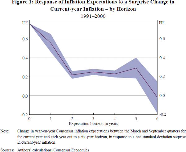
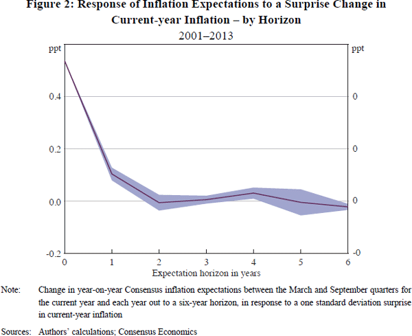
A direct way of seeing one aspect of this change in behaviour is to look at the way long-term inflation expectations respond to inflation surprises. If expectations are well-anchored they should not respond to surprises. On the other hand, if inflation expectations are adaptive or otherwise poorly anchored one would expect to see revisions to longer-term expectations when a surprise occurs. To assess this we use Consensus Economics forecasts of inflation and look at the way expectations change between the March and September quarters. The change in current year inflation expectations between these two dates is a good indicator of the inflation surprise between those dates. Reflecting our comparative advantage, we conduct this exercise on Australian expectations – results for other countries are similar.[1]
Formally, for forecast horizons up to six years ahead, we estimate the regression
where  is the September quarter Consensus forecast in year
t for inflation in year t + h, and similarly for
the other forecast terms in the regression. The coefficient βh
is the estimated revision to inflation expectations at horizon h in
response to a surprise in current-year inflation.
Data are available from 1991, so we split the sample approximately in half, with
a sample from 1991 to 2000 that covers the initial years of inflation targeting
in Australia and a sample from 2001 to 2013 reflecting more recent experience.
We estimate regression coefficients βh for each sample period, and show in Figures 1 and
2 the response of inflation expectations to a one standard deviation surprise
in current-year inflation:  .
In the pre-2000 period for Australia, a one standard deviation surprise (March
to September) in current-year inflation tended to raise professional forecasters'
inflation expectations at a five-year horizon, but in the post-2000 period
inflation surprises have had a negligible effect on expectations (abstracting
from base effects). Inflation expectations are clearly better anchored today
than they were when inflation targeting was first being established in Australia.
While this evidence is relatively direct and transparent, it is only partial. There are other ways in which inflation targeting may have affected the behaviour of inflation. For example, there is ongoing debate about whether the relationship between economic slack and inflation has been changing or, conversely, whether more stable inflation has been a sign of small levels of economic slack despite heightened unemployment.[2] Furthermore, particularly in small open economies, there has been a debate about the changing influence of imported goods and services prices on domestic inflation. To address these issues in a more comprehensive way, we estimate a relatively standard New-Keynesian Phillips curve. To allow for the fact that the inflation process may have changed over time, we estimate a model with time-varying parameters using a non-linear Kalman filter developed by Matheson and Stavrev (2013). This framework allows us to simultaneously examine changes in the slope of the Phillips curve, the degree of anchoring in inflation expectations, and the level of the non-accelerating inflation rate of unemployment (NAIRU).
More technically, in our estimation annualised inflation πt is described by a Phillips curve that depends on
inflation expectations  , the deviation of unemployment from its natural rate
(ut −
  ),
and import price inflation
  :
:
The import price term is demeaned tariff-adjusted import price inflation relative to CPI inflation, in year-ended terms. Inflation expectations is a weighted average of a forward-looking measure, long-term Consensus inflation expectations, and a backward-looking measure, lagged year-ended inflation:[3]
The unemployment gap evolves according to the first-order autoregressive process
with the NAIRU evolving according to a random walk process:
The shock  is interpreted to be a demand shock, and
  a shock to the level
of the natural rate of unemployment. The slope of the Phillips curve kt
≥ 0, the weight on long-term inflation expectations 1 ≥ θt
≥ 0, and the coefficient on import prices γt ≥
0 are time-varying, each evolving according to a constrained random walk. The
coefficient ρ is constant throughout the sample period.
The natural rate of unemployment and time-varying parameters are treated as unobserved states, and estimated using a constrained non-linear Kalman filter. A non-linear Kalman filter is required because the measurement equation is multiplicative in unknown state variables: the natural rate of unemployment and the coefficient on the unemployment gap are both allowed to be time-varying.
Initial values for the shock variances are calculated using 10-year rolling non-linear
least squares regressions, with the parameters and the natural rate of unemployment
assumed to be constant within each 10-year window. Constrained maximum likelihood
is used to estimate the parameter ρ and the shock variances, subject to the constraint that the
estimated shock variances are no larger than across the 10-year rolling windows.
Because there is a potential identification problem for the unemployment gap
demand shock  and the natural rate shock
 , the relative variance of these two shocks is imposed. We follow Matheson and
Stavrev (2013) in choosing S ≡ VAR
  /var
/var equal to 15, resulting
in relatively stable estimates for the natural rate of unemployment; for robustness
we also estimate the model assuming S = 5, which results in a relatively
flexible NAIRU (shown on Figure 3 but the corresponding parameter estimates
are omitted on Figures 4–6 for clarity – they are qualitatively
similar to those
shown).[4]
We estimate the system at a quarterly frequency for the period 1965–2013, using
CPI inflation excluding interest charges and health and tax policy
changes.[5]
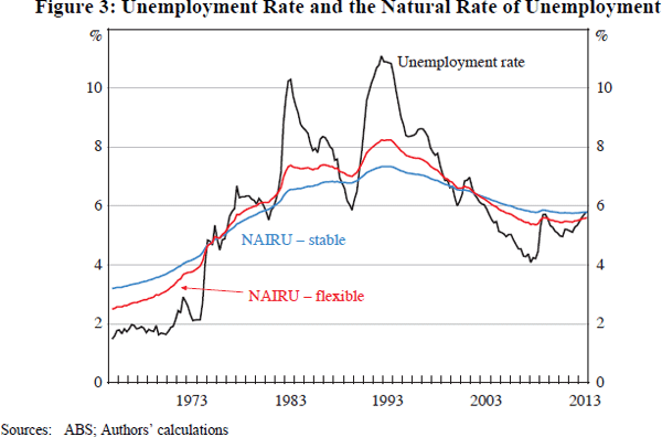
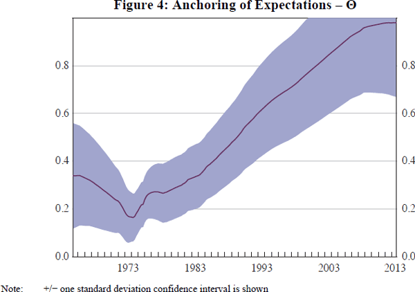
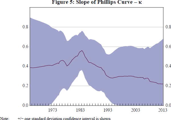
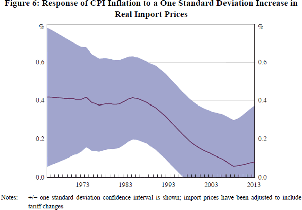
Figures 3–6 report the two-sided smoothed estimates of the natural rate of unemployment and the slope parameters. The estimated NAIRU depends on the imposed degree of stability, and so the size of the unemployment gap at any point in time is quite uncertain, the more so at the end points. To give a sense of the uncertainty inherent in these estimates, we present two such estimates in Figure 3. Furthermore, as we discuss later, changes in the inflation process have made it much more difficult to estimate the NAIRU precisely. As such, little weight should be placed on the particular estimates of the NAIRU shown here. For our purposes, the important aspect of these estimates is that we use a NAIRU that is internally consistent; the estimates of the other parameters are not particularly affected by the degree of smoothness we impose on the NAIRU.
Turning to the parameters of most interest, we see that, following the introduction of inflation targeting, inflation has become more firmly anchored on long-term expectations, and less on the previous year's inflation rate: the coefficient θt on long-term bond market inflation expectations has risen toward unity over the inflation-targeting period. Furthermore, since the introduction of inflation targeting, long-term inflation expectations have themselves become better anchored: since 1998, long-term inflation expectations have never deviated from the midpoint of the RBA's inflation target by more than 0.2 percentage points, unlike in earlier years when co-movement between long-term expectations and current inflation was clearly evident. At the same time, the coefficient kt on the unemployment gap has become smaller, indicating a flattening of the Phillips curve. Although tradeable inflation now accounts for a larger share of overall inflation variability, the speed with which import price changes pass through to consumer price changes appears to have slowed. In particular, Figure 6 shows that the effect on consumer price inflation of a one standard deviation increase in year-ended import price inflation is estimated to have declined over the inflation-targeting period.
Our econometric results suggest that shocks have much less of an effect on inflation now than prior to the introduction of inflation targeting. The wage-price spirals that economists of the 1970s worried about seem to be less of a concern today, reflecting better-anchored inflation expectations, but also decentralisation of the wage-bargaining process. The transitory nature of inflation surprises in an inflation-targeting world is confirmed by a trend-cycle decomposition of inflation. For the United States, Stock and Watson (2007) show that the variance of the trend component of inflation declined sharply in the mid 1980s, following the Volcker disinflation, and declined further after 1990, falling to a level of volatility not seen since the mid 1950s. Variability in the transitory component is largely beyond the control of central banks, and has remained unchanged. Thus, the share of inflation variability accounted for by transitory shocks has risen sharply.
For Australia, a simple way to see this change in the inflation process is to compare tradeable and non-tradeable inflation between the 1980s and 1990s, when inflation targeting was in its infancy, and today. Although tradeable inflation includes a domestic retailing component, a large portion of the variation in tradeable goods and services prices reflects external influences. Consistent with the results of Stock and Watson (2007) for the United States, the first panel in Table 1 indicates that there has been a negligible change in the variance of tradeable inflation in the pre- and post-inflation targeting periods. (We exclude the disinflationary period from these calculations to guard against attributing the mean shift in inflation to variability in the pre-inflation targeting period.) In contrast, the variance of non-tradeable inflation – the set of prices influenced by Australian monetary policy – has fallen by more than half. Compounding the increase in the relative importance of imported inflation, the covariance between tradeable and non-tradeable inflation has declined between the pre- and post-inflation targeting periods. The persistence of non-tradeable inflation has fallen together with its variance between the pre- and post-inflation targeting periods: the sum of the autoregressive coefficients for non-tradeable inflation falls from 0.44 in the pre-inflation targeting period to 0.21 in the post-inflation targeting period (see the second panel in Table 1). Consistent with our earlier results, the variance of shocks to non-tradeable inflation, estimated by the residuals of the autoregressive models for the pre- and post-inflation targeting periods, has fallen substantially. There is little evidence of persistence in tradeable inflation in the pre- or post-inflation targeting periods.
| Pre-inflation targeting |
Post-inflation targeting |
||
|---|---|---|---|
| 1982:Q2–1990:Q4 | 1993:Q1–2013:Q4 | ||
| Original series | Variance: non-tradeables | 0.90 | 0.15 |
| Variance: tradeables | 0.60 | 0.58 | |
| Covariance | 0.31 | −0.02 | |
| Autoregressive model: p-lags | |||
| Non-tradeables | Sum of coefficients | AR(1): 0.44 | AR(4): 0.21 |
| Variance of residuals | 0.69 | 0.12 | |
| Tradeables | Sum of coefficients | AR(0): 0 | AR(2): −0.16 |
| Variance of residuals | 0.60 | 0.49 | |
| Covariance of residuals | 0.22 | −0.03 | |
| Notes: Data are in percentage points, at a quarterly frequency, excluding tax changes and interest charges; lag lengths were selected using the AIC criterion | |||
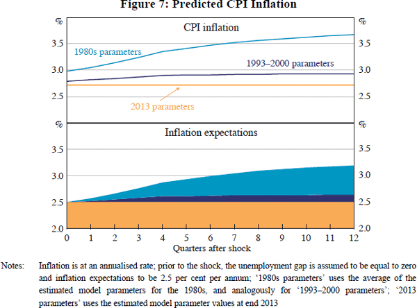
Associated with these changes, the relationship between unemployment and inflation has become substantially weaker. To illustrate the flattening of the Phillips curve, we forecast the response of inflation under old and current parameter values to a sustained one percentage point deviation in unemployment below its natural rate. Figure 7 indicates that the predicted response of inflation to an unemployment gap is now smaller than under parameter values estimated prior to and in the early years of inflation targeting. Inflation is less sensitive to an unemployment gap than in the past for two reasons: first, the slope of the Phillips curve has declined, and second, because inflation expectations are now firmly anchored on the inflation target, the increase in inflation caused by the unemployment gap has a negligible effect on inflation expectations.[6] The contribution of inflation expectations to predicted CPI inflation for each scenario is indicated by the shaded areas in Figure 7. The sensitivity of inflation to import prices is also estimated to have declined, although our scenario assumes unchanged import prices.
With a flatter Phillips curve, much of the variability in inflation is now dominated by transitory changes, and deviations in unemployment from its natural rate are more difficult to detect in inflation data than in the past. Excess demand pressures are more likely to be swamped by noise than in previous decades. Conversely, changes in unemployment and output are less useful for forecasting inflation than in the past. In a particularly stark demonstration of this point, Atkeson and Ohanian (2001) found NAIRU-based inflation forecasts to now be little better than naïve inflation forecasts of US inflation. For Australia, this was demonstrated by Heath, Roberts and Bullman (2004).
Footnotes
See IMF (2011). [1]
See Debelle and Vickery (1997) and Kuttner and Robinson (2008). [2]
After 1991, the long-term inflation expectations series is Consensus' forecasts for CPI inflation 6–10 years ahead; expectations are surveyed in the June and December quarters, and we linearly interpolate between observations. From 1986 to 1991, we use long-term inflation expectations implied by inflation-indexed bonds, and before 1986 expectations are proxied by the difference between 10-year nominal bonds and an estimate of the world real interest rate (see Debelle and Laxton (1997)). [3]
To avoid convergence on unrealistic variances for the shock processes when S = 5, we restrict the estimated variances of the shocks to the parameters kt, θt and γt to be no less than one-quarter of their estimated magnitude in 10-year rolling regressions; at an optimum, these constraints do not bind. [4]
The official target measure for Australia used Treasury underlying inflation between 1993 and 1998; the econometric results are similar using Treasury underlying inflation in place of CPI inflation for this period. [5]
We assume long-term inflation expectations remain anchored at target, which we believe is reasonable provided deviations from the inflation target caused by policy errors are rare. [6]


