RDP 2015-06: Credit Losses at Australian Banks: 1980–2013 4. Econometric Analysis
May 2015 – ISSN 1448-5109 (Online)
- Download the Paper 1.46MB
The narrative account in Section 3 reveals a range of features of credit losses in Australian banking. Aggregate credit losses clearly have a relationship with the economic cycle, but appear to be affected by macro-level factors other than just output growth. Business sector conditions, such as commercial property prices and business indebtedness, look to have played the key role. The composition of banks' portfolios also appears important: credit losses look to have been incurred mainly on business lending. But the direct evidence for this is based on data from only a few banks for the largest episode of credit losses. Cross-sectional differences in bank-level credit losses have been large, and there are suggestions that these are driven by variation in lending standards (as well as portfolio composition). Section 4 uses a panel data modelling framework to explore these issues further.
4.1 Modelling Approach
Consistent with the international literature, I model the relationships between bank-level credit losses and both macro-level and bank-level factors (see Equation (1)).[16] I use annual bank-level current loss ratios as the dependent variable (CLRit, where i indexes banks and t years). Following the majority of the literature, I use the fixed-effects (within) estimator, which removes time-invariant bank-level heterogeneity (αi). This is done on the basis that some of this heterogeneity is unobservable and may be correlated with the explanatory variables of interest. Relevant unobservables include the average risk appetite of a bank's managers and, relatedly, its average lending standards (both of these probably also vary within banks over time, and this is explored in Section 4.4).

Macro-level explanatory variables (MACROt) include real GDP growth, growth in business sector profits and growth in the household sector's disposable income, all measures of changes in borrowers' incomes. The level of the cash rate, as well as the interest burdens of the whole economy, household sector and business sector, are included as more precise measures of borrowers' ability to repay their loans.[17] System-wide nominal credit growth, and growth in nominal housing and business credit, are intended to capture system-wide changes in lending standards (see, for example, Keeton (1999)). Residential and commercial property are used as collateral for housing and business loans in Australia, so changes in the prices of these assets are included to capture changes in the value of this collateral. Details of variable construction, descriptive statistics and correlations for all explanatory variables are in Appendix B (Tables B2, B3 and B4).
Bank-level variables (BLEVELit) include the shares of each bank's portfolio devoted to business and personal lending, and bank-level loan growth.
I include all variables contemporaneously, except for interest burden (which I lag one year) and the credit and loan growth variables (I include lagged terms covering the past four years for these variables). These variables are excluded contemporaneously because of the mechanical impact of credit losses on the level of credit and loans (these measures are calculated net of identified losses). I exclude bank-year observations on banks making up less than 1 per cent of total bank loans to prevent idiosyncratic risk in very small loan portfolios from clouding my results. This leaves 328 observations on 26 banks covering 1982 to 2013.
4.2 Initial Models
Table 1 reports regression results from two alternative forms of Equation (1). Model A uses mainly economy-wide macro-level explanatory variables. Model B uses variables specific to the household and business sectors.
These models indicate that the drivers of credit losses over 1982–2013 are largely those highlighted by previous Australian work using shorter time periods. At the macro level, interest burdens, sectoral credit growth measures, and growth in residential and commercial property prices appear to influence losses, and measures specific to both the business and household sectors appear important. These results are entirely consistent with Gizycki (2001), who modelled ex post credit risk at Australian banks over periods ending in 1999. Banks with mainly business lending appear to have incurred higher credit loss rates than banks with mainly housing lending, in line with Esho and Liaw (2002). The model that uses only sectoral macro-level variables (Model B) explains credit losses slightly better than the one that uses primarily economy-wide variables (Model A). This is useful for the development of the main model of this paper – presented in Section 4.3 – which includes interactions between portfolio shares and macro-level variables.
| Variable | Model A | Model B |
|---|---|---|
| Macro-level | ||
| GDP growtht | −0.063* | |
| Business profits growtht | −0.041*** | |
| Household disposable income growtht | −0.006 | |
| Cash ratet | −0.007 | |
| Economy-wide interest burdent − 1 | 0.137*** | |
| Business sector interest burdent − 1 | 0.062** | |
| Household sector interest burdent − 1 | 0.144*** | |
| Commercial property price growtht | −0.020*** | −0.006 |
| Residential property price growtht | −0.016*** | −0.012*** |
| Credit growtht − 1 | −0.012 | |
| Credit growtht − 2 | −0.023 | |
| Credit growtht − 3 | 0.026 | |
| Credit growtht − 4 | −0.024 | |
| Business credit growtht − 1 | −0.028*** | |
| Business credit growtht − 2 | −0.007 | |
| Business credit growtht − 3 | 0.028* | |
| Business credit growtht − 4 | −0.019* | |
| Housing credit growtht − 1 | 0.032*** | |
| Housing credit growtht − 2 | 0.013 | |
| Housing credit growtht − 3 | −0.025 | |
| Housing credit growtht − 4 | 0.007 | |
| Constant | −1.576*** | −2.749*** |
| Bank-level | ||
| Business share of lendingt − 1 | 2.087** | 2.241** |
| Personal share of lendingt − 1 | 3.254*** | 3.337*** |
| Loan growtht − 1 | 0.009 | 0.006 |
| Loan growtht − 2 | 0.008* | 0.005 |
| Loan growtht − 3 | 0.001 | 0.001 |
| Loan growtht − 4 | 0.013** | 0.011** |
| Observations | 328 | 328 |
| Within R-squared | 0.48 | 0.54 |
| Adjusted within R-squared | 0.45 | 0.51 |
| AIC | 725 | 697 |
| BIC | 785 | 781 |
| Notes: All models are estimated with bank fixed effects and standard errors are clustered by bank; ***, ** and * denote significance at the 1, 5 and 10 per cent level respectively | ||
These simple models offer a number of other insights:
- Looking first at the proxies for borrower income, GDP growth is intuitively signed, but only significant at the 10 per cent level. Output growth has been found insignificant in international studies using models that include a range of cyclical macro-level variables (Davis and Zhu 2009). At the sectoral level, business profits growth has a negative relationship with credit losses that is significant at the 1 per cent level, while growth in household disposable income does not appear to be a significant explanator of credit losses. This difference is consistent with the relative importance of developments in these sectors in the narrative account of credit losses in Australia.
- The economy-wide interest burden has a statistically significant relationship with credit losses in Model A. A one standard deviation increase in this variable (roughly 2 percentage points) is associated with a 26 basis point rise in credit loss ratios. The economy-wide aggregate interest burden is the weighted average of borrower-level interest burdens across the economy; a rise in the former must represent some increase in risk at the borrower level. Interest burdens within both the business and household sectors appear to underlie this aggregate relationship – both are significant in Model B. This is consistent with Gizycki (2001), but is not consistent with the narrative account of credit losses in Australia. Default and financial distress among household borrowers does not feature prominently in this.
- Both residential and commercial property price growth appear to influence bank credit losses. Again, while consistent with Gizycki (2001), this is not entirely consistent with the narrative account of credit losses in Australia. Residential property has primarily served as collateral for housing loans in Australia, and the available evidence indicates banks have not incurred significant credit losses on such loans over recent decades. Residential property now also collateralises a significant amount of small business lending in Australia, but this makes up only a small proportion of total business lending and it is unclear how prevalent this arrangement was in earlier decades.
- Business credit growth and housing credit growth are important for credit losses in this model, though they have opposite effects over short horizons. Positive relationships between longer lags of credit and loan growth and losses are the most common finding in the international literature, and are generally thought to operate through increases in credit supply that involve lending to less financially sound borrowers (see Section 4.4). Though there is an explanation for the estimated negative relationship between business credit growth and losses – more easily available credit (signalled by strong credit growth one year ago) may make refinancing easier for weaker borrowers who would otherwise default – this estimated relationship should be interpreted cautiously. Demand for credit probably weakens during downturns (which in turn cause credit losses), so the estimated relationship may not be causal.
- At the bank level, portfolio composition has statistically significant effects with relative magnitudes that accord with the portfolio-level loss rates shown in Section 3.1.2. A bank with more business lending and less housing lending incurs higher credit losses. More (non-housing) personal lending has a similar, but stronger, effect. Higher loan growth raises losses at the individual bank level with a multi-year lag. The estimated coefficients on this variable are of a similar magnitude to those found by Hess et al (2009) for Australian banks.
4.3 Using Portfolio Composition
This section contains the primary econometric model for credit losses presented in this paper. It uses the same modelling framework as the simple models presented in Section 4.2, but relies on explanatory variables that are interactions between macro-level variables and bank-level portfolio shares. Equation (2) shows a model of this type: BSLit − 1 is the share of bank i's lending that was business lending at t − 1, and MACRO1t contains macro-level variables likely to affect credit losses on business lending (HSLit − 1 and MACRO2t are defined analogously for housing lending, and PSLit − 1 and MACRO3t for personal lending). The model uses all of the macro-level variables in Model B above. Those assigned to MACRO1t are simply those thought to cause credit losses on business lending: business profits growth, the business sector interest burden, business credit growth, and commercial property price growth. The other macro-level variables – those that capture the conditions in the household sector – are present in both MACRO2t and MACRO3t, except for housing credit growth, which is in MACRO2t only.

The key idea is that requiring macro-level variables to affect credit losses through the portfolios they are related to should provide better identification of the drivers of credit losses. For example, the mechanism through which falls in residential property prices are thought to cause credit losses is by lowering the value of the collateral backing housing loans. A model that requires changes in residential property prices to act on credit losses through banks' housing lending should distinguish this causal channel from mere correlation between house prices and other macro-level conditions that cause credit losses (cross-correlations between my explanatory variables are shown in Appendix B). The limited international literature that models credit losses at the portfolio level generally finds each portfolio has a different relationship with macro-level conditions.[18]
A necessary condition for the unbiased estimation of Equation (2) is that the portfolio shares are independent of the error term. One reason why this assumption may not hold is correlation between (within-portfolio) lending standards and portfolio shares. But arguments can be made for both positive and negative relationships; banks that do more business lending should be better at selecting businesses to lend to, but banks with a lot of business lending may have arrived at that position by accepting borrowers other banks did not. The dataset contains a wide range of variation in portfolio composition, in part due to the regulatory distinctions between savings banks (which mainly concentrated on housing lending) and trading banks (which mainly concentrated on business lending) over the late 1980s and early 1990s. The state government-owned banks that received extraordinary government support in the early 1990s had shares of business lending in the middle of the sample range.
Table 2 shows the estimation results from the model (Model C). The key insight from Model C is that business sector conditions appear to have been the main driver of credit losses in Australia over recent decades. The household sector interest burden, residential property prices, and housing credit growth no longer have significant relationships with credit losses when required to interact with credit losses through household lending. In other words, studies showing macro-level correlations between measures of household sector financial conditions (such as housing prices) and future financial crises might actually be picking up a correlation between housing prices and the actual drivers of financial distress, not a causal link from housing prices to financial instability.
| Variable | Interacted with(a): | Model C |
|---|---|---|
| Macro-level | ||
| Business profits growtht | BSL | −0.072*** |
| Household disposable income growtht | HSL | −0.026 |
| Household disposable income growtht | PSL | 0.118 |
| Business sector interest burdent − 1 | BSL | 0.128*** |
| Household sector interest burdent − 1 | HSL | 0.048 |
| Household sector interest burdent − 1 | PSL | 0.105 |
| Commercial property price growtht | BSL | −0.033** |
| Residential property price growtht | HSL | −0.025 |
| Residential property price growtht | PSL | −0.012 |
| Business credit growtht − 1 | BSL | −0.042*** |
| Business credit growtht − 2 | BSL | 0.007 |
| Business credit growtht − 3 | BSL | 0.060* |
| Business credit growtht − 4 | BSL | −0.017 |
| Housing credit growtht − 1 | HSL | 0.019 |
| Housing credit growtht − 2 | HSL | −0.008 |
| Housing credit growtht − 3 | HSL | −0.019 |
| Housing credit growtht − 4 | HSL | 0.003 |
| Constant | −0.183 | |
| Bank-level | ||
| Business share of lendingt − 1 | −0.907 | |
| Personal share of lendingt − 1 | 0.279 | |
| Loan growtht − 1 | 0.006 | |
| Loan growtht − 2 | 0.001 | |
| Loan growtht − 3 | −0.004 | |
| Loan growtht − 4 | 0.009* | |
| Observations | 328 | |
| Within R-squared | 0.62 | |
| Adjusted within R-squared | 0.58 | |
| AIC | 642 | |
| BIC | 733 | |
|
Notes: Model C is estimated with bank fixed effects and standard errors are clustered
by bank; ***, ** and * denote significance at the 1, 5 and 10 per cent
level respectively (a) BSL = business share of lending, HSL = housing share of lending and PSL = personal share of lending; portfolio measures used in interactions are lagged one period |
||
Business profits growth, the business sector interest burden, business credit growth, and commercial property price growth are all significant at the 5 per cent level in Model C. This model also has a better statistical fit than Models A and B, indicating that incorporating portfolio interactions is a valid choice.
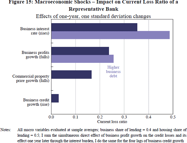
Most of the statistically significant relationships in Model C are economically significant. The median, mean and standard deviation of current losses in the dataset used for this regression are 24, 57 and 107 basis points respectively, and one standard deviation changes in key macro-level variables generate losses that range from 3 basis points to 49 basis points (the dark bars in Figure 15).[19] Changes in business interest rates and business profit growth appear to be the most important for credit losses. Both affect losses through changes in the business sector interest burden, as well as directly in the case of business profits. The model implies that the level of business debt relative to interest rates and profitability is an important state variable for losses. Assuming an initial business sector interest burden equal to the average over 1981–90 (21.4 per cent), rather than the sample average (16.4 per cent), leads to the larger effects on losses shown by the lighter bars in Figure 15.
Another way to look at the influence of macro-level variables is to examine the contribution of each variable to the aggregate current loss ratio predicted by Model C. Figure 16 plots the contribution of each macro-level variable and its interacted portfolio share to the CLR of the whole sample in each year.[20] The contributions of all household macro-level variables are shown as an aggregate, as are the contributions of the variables in the model that are not interacted with macro-level variables.[21] The aggregate level of credit losses predicted by Model C fits actual losses quite closely (the RMSE is 0.15), so this model provides a macro-level explanation that, while suffering from the same limitations as all models, quite closely fits the actual experience.
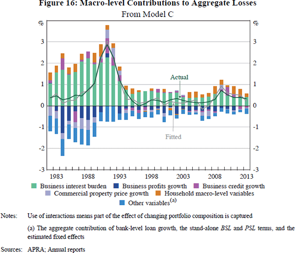
The key take-away from this decomposition is that business sector conditions have been the macro-level driver of aggregate credit losses (as they have been for bank-level credit losses). Household macro-level variables, even in aggregate, have made only small contributions to changes in the aggregate CLR. Rising business indebtedness placed upward pressure on credit losses during the first decade of the sample. During the 1980s, this was offset by fast growth in business profits and commercial property prices. Slowing growth in (and eventually falls in) profits and commercial property prices, in combination with the high business sector interest burden, triggered the large rises in credit losses in the early 1990s. A similar, but smaller, dynamic underlies the rise in the fitted CLR between 2007 and 2009. During both episodes, sharp slowdowns in business credit growth also contributed to higher aggregate losses.
By construction, Figure 16 attributes most of the variation in aggregate credit losses to macro-level variables, as it aggregates the contribution of changes in each macro-level variable and changes in the portfolio share with which it is interacted. Figure 17 takes the alternative approach of applying changes in macro-level variables while holding the banking system constant. This is done for two reference years, 1991 and 2008. For example, the line for 1991 shows the aggregate CLR predicted by Model C for the 16 banks in the sample in 1991, applying the actual macro-level variables experienced in each year, but freezing each bank's portfolio composition and past loan growth at 1991 values. The distance between each of counterfactual lines and the actual fitted values from Model C shows how changes in the banks in the sample, and their characteristics (from the reference year), contribute to aggregate losses.
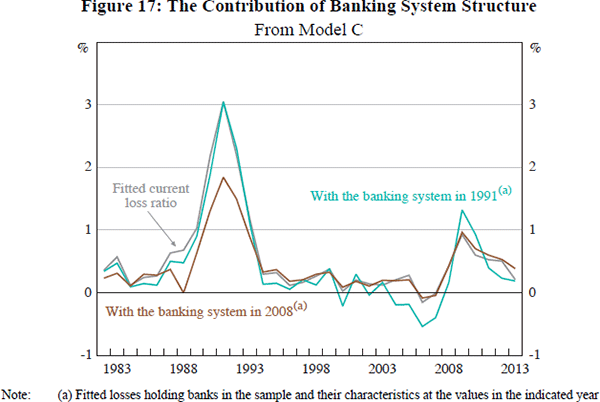
Figure 17 indicates that different macro-level experiences do not explain all of the difference in credit losses between the early 1990s and global financial crisis episodes. For example, the banking system in 2008, if subjected to the macro-level conditions present in the early 1990s, is predicted to incur credit losses of around 5½ per cent over the period (the area under the 2008 line between 1990 and 1994). This is 3 percentage points below the actual credit loss ratio incurred over this period.[22] A reasonable conclusion is that both changes in the macroeconomic environment and changes in the structure of the banking system explain the large difference in credit losses between the early 1990s and global financial crisis episodes.
Caution should be used in giving causal interpretations to the relationships estimated by these econometric models. While most of the estimated relationships are intuitive – the business sector interest burden, for example, has a very natural relationship with credit losses – reverse causality may be present. A good example of this is the United States during the global financial crisis, where credit losses on residential mortgages destabilised large financial intermediaries with consequent impacts upon broader economic and financial conditions (Hall 2010; Mishkin 2011). This causal chain is likely to have been less important in Australia during my sample period, mainly because of the robust position of the Australian banking system over the whole period (including while it was subject to large credit losses in the early 1990s). This argument is not that there is no casual channel from credit losses to macroeconomic conditions in Australia, but rather that it was not triggered during my sample period. Public actions during crisis periods have also dampened this channel in Australia.
The results of Model C are robust to a number of alternative specifications, including alternative portfolio interactions, alternative lag structures, and different sample periods (see Section C.1 of Appendix C). Omitted variable bias is probably the greatest statistical concern: lending standards have not been discussed in the context of the models, but are likely very important for credit losses.
4.4 Lending Standards
The econometric models above treat all business lending as having equal propensity to cause credit losses (conditional on the macroeconomic environment), regardless of whether it is business lending in the early 1990s or in the mid 2000s, and regardless of the bank doing the lending. But there is evidence that this is not an accurate assumption; that, for example, lending standards were worse in the late 1980s than in the early 2000s. And, internationally, empirical work has shown that lending standards vary over time and played a role in the global financial crisis (see, for example, Lown, Morgan and Rohatgi (2000); Maddaloni and Peydró (2011); and Dell'Ariccia, Igan and Laeven (2012)). This section of the paper attempts to quantitatively explore the effect lending standards have had on credit losses in Australia.
Lending standards, particularly for lending to businesses, are not well-defined in the literature. The definition I employ is given in Section 3.1.1: non-price differences in borrower characteristics and loan terms that are ex ante observable by a bank. Importantly, I do not include portfolio composition at the level of business, housing and personal lending as a component of lending standards. Some examples of changing lending standards were given in Section 3.1.1. But my definition encompasses other differences, such as the industry composition of a bank's business lending. A business lending portfolio with a higher share of commercial property lending, which has historically been riskier than other business lending (Ellis and Naughtin 2010), could be described as of a lower standard under my definition.
Changes in average lending standards over time are captured reasonably well by Model C, given its close fit at the aggregate level. Several of the macro-level variables in this model likely act as proxies for lending standards. As shown in Figure 15, the long-run relationship between business credit growth and credit losses is positive, and this probably captures increases in credit supply that involve lending to less financially sound borrowers (see, for example, Keeton (1999)). Jiménez and Saurina (2006) use loan-level data to show that, controlling for macroeconomic conditions, loans originated while a bank is growing faster are more likely to default and less likely to be collateralised.
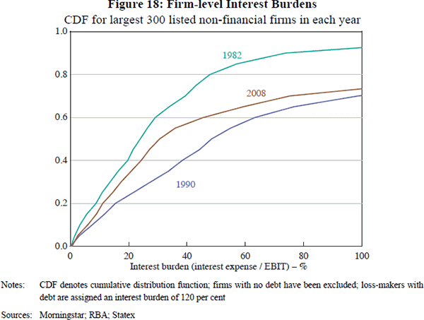
The business sector interest burden is also likely acting as a proxy for average lending standards. Banks extending business loans often place a contractual limit upon businesses' interest burdens (at origination and/or over time). The aggregate business sector interest burden, the weighted average of the interest burdens of all businesses in the economy, captures some portion of the time series variation in this lending standard. Firm-level data illustrate this clearly. Looking at the largest 300 listed companies at each point in time, firm-level interest burdens were higher in 1990 than in either 1982 or 2008 (Figure 18). For example, around half of the largest 300 listed firms had an interest burden above 50 per cent in 1990, while less than one-fifth of the largest 300 listed firms in 1982 had an interest burden above this level. This variation is partly captured by the aggregate business sector interest burden, which was 17.0, 28.4 and 16.2 in 1982, 1990 and 2008.[23] The firm-level ranking also correlates with the relative magnitudes of the credit losses experienced during the downturns that began in each of these years.
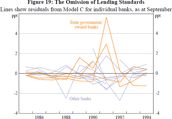
In contrast, Model C does a poor job of explaining cross-sectional variation in lending standards. Model residuals during the early 1990s are very large for some state government-owned banks, and the narrative evidence presented in Section 3 indicates that these banks had below-average lending standards (Figure 19). The bank-level variables included in Model C, portfolio composition and bank-level loan growth, do not explain why the credit loss ratios experienced by these banks were so much larger than those at other banks. This omission of lending standards is partly responsible for the higher RMSE of Model C at the bank level: this statistic drops from 63 to 44 basis points if state government-owned banks are excluded.
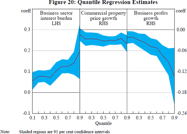
There has almost certainly been more variation in lending standards than is indicated by this state government-owned/non-state government-owned distinction. But little other hard information on lending standards is available. Quantile regression is one strategy that has been used to assess the effect of unobserved heterogeneity in other areas of economics.[24] This method models the distribution of credit losses, conditional on the explanatory variables. It provides a more complete description of relationships than least squares regression, which is based upon estimating only the conditional mean of a dependent variable. If unobserved differences in lending standards are the primary determinant of the conditional distribution of credit losses, estimated relationships with macro-level variables at higher (lower) quantiles can be interpreted as being for banks with worse (better) lending standards. If other factors (e.g. idiosyncratic risk) are the primary determinants of the conditional distribution of credit losses, this interpretation does not hold and quantile regression estimates merely show the range of possible responses to changes in macro-level variables.
Quantile regression is also more robust to outlier observations than least squares methods (Cameron and Trivedi 2009). For example, the significance of commercial property prices in the above models could be driven entirely by a very strong relationship for a subset of banks that experienced credit losses well above-average. But in a quantile regression, this should be apparent in the lack of a relationship between the variables and some parts of the credit losses distribution.
Quantile regression generates estimated relationships with macro-level variables that vary widely across the distribution, and do so in a way that is statistically significant in some cases (Figure 20; full quantile regression outputs are in Table C1).[25] Notably, key macro-level variables are estimated to have statistically significant effects, signed in line with estimated coefficients in Model C, on losses across almost all of the distribution. For example, the effect of the business sector interest burden upon losses at the 90th percentile is more than three times as large as at the 10th percentile. More concretely, a one standard deviation rise in business sector interest burden (5.5 percentage points) raises credit losses by 12 basis points at the 10th decile of the distribution, while it raises credit losses by 43 basis points at the 9th decile (for a bank with 40 per cent business lending). The comparable impact from Model C is 30 basis points.
Footnotes
A survey is available in Glogowski (2008). Salas and Saurina (2002) are a commonly cited precedent when using macroeconomic and bank-level explanatory variables to model bank-level credit risk outcomes. [16]
The economy-wide interest burden is equal to the estimated interest payments on all intermediated debt in the economy divided by GDP. The business and household sector interest burdens are defined similarly: see Table B2. [17]
For example, using data on Greek banks, Louzis, Vouldis and Metaxas (2012) found non-performing personal loans to be very sensitive to interest rates, business lending sensitive to GDP growth, and mortgages not very sensitive to macroeconomic developments. Hoggarth, Logan and Zicchino (2005) estimate models for sectoral write-offs from UK banks' business, personal, and housing portfolios that are each driven by a different set of macro-level variables. [18]
Sample means used in Figure 15 are: business interest burden (16.4 per cent), business interest rate (10.5 per cent), commercial property price growth (5.2 per cent), business profits growth (7.4 per cent), and business credit growth (10.8 per cent). One standard deviation shocks are: business interest rate (+4.5 percentage points), commercial property price growth (−12.3 percentage points), business profit growth (−6.1 percentage points), and business credit growth (+9.5 percentage points). [19]
As an example, the contribution of commercial property price growth (CPPG) in 1991 is:  , where A is the set of banks in
the sample in 1991, and ωi,1990 the appropriate
weight for each bank (each bank's share of sample loans, based on loans
outstanding in 1990).
[20]
, where A is the set of banks in
the sample in 1991, and ωi,1990 the appropriate
weight for each bank (each bank's share of sample loans, based on loans
outstanding in 1990).
[20]
This is shown as the ‘Other variables’ contribution in Figure 16. [21]
An alternative estimate is the area between the 1991 and fitted CLR lines between 2008 and 2012. This is smaller (around ½ percentage point). The large difference between these estimates is an inherent drawback of the structure of Model C. [22]
The aggregate and firm-level measures differ slightly. Aggregate interest burden captures interest on intermediated debt only, while the firm-level measure captures interest on all debt. The aggregate measures of business profits, gross operating surplus (for private non-financial corporates) and gross mixed income (for unincorporated enterprises) differ somewhat from the firm-level measure, earnings before interest and tax. [23]
Bitler, Gelbach and Hoynes (2006), for example, examine quantile treatment effects in a labour economics context. ‘Quantile’ is a synonym for ‘percentile’. [24]
I use a parsimonious version of Model C for the quantile regression, and I drop the fixed effects. [25]