RDP 2015-01: Stress Testing the Australian Household Sector Using the HILDA Survey 4. Method

4.1 Data

The stress-testing model uses data from the HILDA Survey, which is a nationally representative household-based longitudinal study collected annually since 2001. The survey asks questions about household and individual characteristics, financial conditions, employment and wellbeing. Modules providing additional information on household wealth (‘wealth modules’) are available every four years (2002, 2006 and 2010).

In this paper, we heavily rely on information from the HILDA Survey's wealth modules, so the years where these data were collected form the basis of our sample. Imputed responses are used where possible to minimise the number of missing responses and thus to increase the sample size. The total sample size for each year is around 6,500 households. Individual respondent data are used to estimate probabilities of unemployment; this part of the model is based on a sample of around 9,000 individuals each year.

4.2 Model

The model in this paper is comparable to the financial margin approach used in Albacete and Fessler (2010). Figure 2 provides an overview of the model.

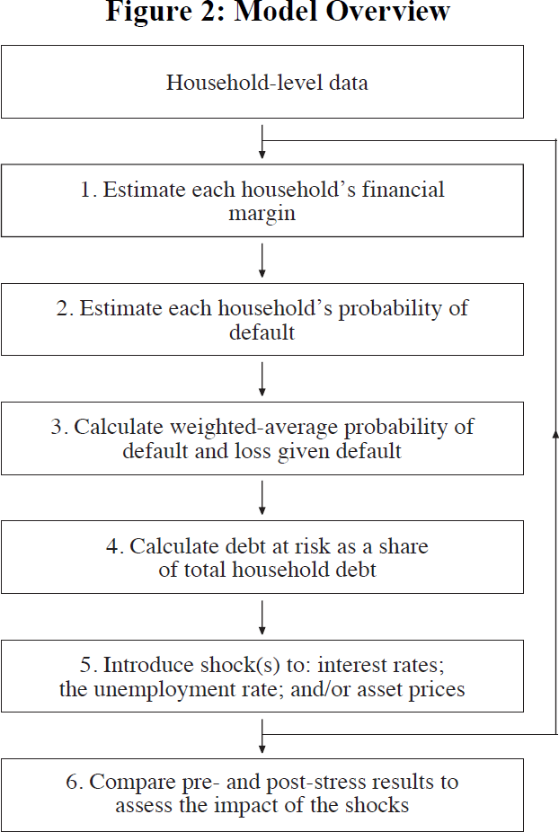
Initially, a pre-stress baseline is established. The first step in calculating this is to estimate a financial margin (FM) for each household (where i subscripts for households):

where Y is household disposable income, DS is minimum debt-servicing costs (if any), MC is minimum consumption expenditure and R is rental payments (if any). All measures are supplied on an annual basis or annualised before inclusion. Disposable income and rental payments are reported in the HILDA Survey. While actual consumption is reported in the survey, minimum consumption is not. However, in a scenario of financial stress, minimum consumption is of greater relevance than actual consumption, as households can reduce discretionary spending to meet their debt obligations. We estimate minimum consumption by mapping values from the Henderson Poverty Line (HPL) to each household based on their characteristics.^[4] Under the HPL, minimum consumption depends on family structure and increases linearly with the number of dependent children.

Minimum debt-servicing costs are estimated as:

where PM is the estimated minimum primary mortgage payment, SM is the reported usual payment on second mortgages,^[5] and P and C are the estimated interest payments on personal and credit card debt, respectively.

The HILDA Survey contains information on ‘usual’ primary mortgage payments; however, this is probably an overestimate of minimum payments, because around half of Australian households pay more principal than required. Instead, minimum primary mortgage payments are estimated using a credit-foncier model, which is a standard financial formula used to calculate mortgage payments on amortising loans. The scheduled loan balance (V) for each household is calculated as:

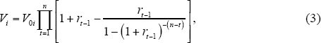
where t is age of the loan in months, V₀ is the household's original loan balance, r is the discounted standard variable interest rate, and n is the initial loan term (which is assumed to be 25 years) in months.^[6] The scheduled balance is used as an input to estimate the minimum monthly primary mortgage payment (w) for each year:

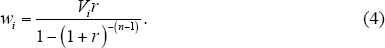
If minimum primary mortgage payments cannot be estimated (due to missing data on key variables), the household's reported usual mortgage payments are used. The estimated minimum annual primary mortgage payment for each year, PM, is obtained by annualising w. Personal and credit card payments are estimated as the product of the reported outstanding balance and average annualised interest rates from that period. This assumes the household does not repay any principal.^[7]

The second step uses the financial margin to calculate each household's probability of default (PD):

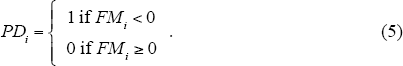
For the purposes of this model, households with a PD of one are assumed to default with certainty. This is a simplification because at least some of these households could draw down on liquid assets or sell property to avoid default. Departures from this assumption are discussed in Section 6.

The third step combines each household's PD with information on debt and assets to calculate the household sector's weighted-average probability of default and loss given default. The weighted-average probability of default (WPD) is:

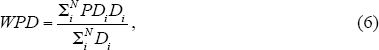
where D is each household's debt and N is the total number of households.

The weighted-average loss given default as a percentage of household debt in default (LGD) is the amount that lenders are unable to recover on defaulted loans:

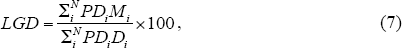
where M_i = max(D_i − A_i, 0) is the dollar value that is lost as a result of a household defaulting, and A is the value of a household's ‘eligible’ collateral – that is, the collateral that lenders would be able to make a claim on in the event of default. Housing loans in Australia are typically full recourse. Hence, in the event of default, lenders have the option of making claims on assets other than the mortgaged property. In practice, however, lenders do not always exercise this option. Throughout this paper, we assume that eligible collateral consists of housing assets only; assuming a broader definition of eligible collateral would result in a lower LGD. Losses are assumed to be borne in order of credit cards, other personal loans and mortgages; this puts downward pressure on LGDs for housing loans and upward pressure for credit card and other personal loans.

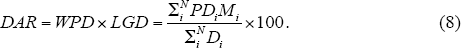
In step four, the WPD and LGD are combined to estimate the weighted-average debt at risk as a share of total household debt (DAR); that is, expected household loan losses flowing through to lenders:

Once the baseline (or pre-stress) results are established, macroeconomic shocks are applied individually or in combination to obtain post-stress results. The difference between the pre- and post-stress results quantifies the impact of the shock in the model. The process is repeated for the three years.

The simulation in this paper in effect assumes that shocks occur instantaneously. As a result, the shocks within the model are difficult to directly compare to real-world shocks, such as a prolonged downturn that involves a long period of high unemployment. In addition, only the first-round effects of the shocks are analysed. The effect of the shocks may be larger or smaller in a multi-period framework. They would also probably be larger if second-round or contagion effects were taken into account.

Footnotes

The HPL estimates the minimum income level required to avoid a situation of poverty for a range of family sizes and circumstances. Some lenders use this measure of household living expenses in their assessments of loan serviceability for new borrowers. In recent years, many lenders have moved away from the HPL toward the Household Expenditure Measure (HEM), which was designed to be a more accurate estimate of living expenses. Overall, although the results can be heavily influenced by the assumptions about minimum consumption, the difference between the HPL and the HEM is small enough to have only a minor effect. [4]

The survey contains insufficient information to calculate minimum secondary mortgage repayments. Hence, reported usual repayments are used. [5]

The month in which a loan is taken out is not available in the dataset, so we assume that all loans were taken out in September. [6]

The HILDA Survey includes personal loan payment data in the 2002 and 2006 surveys, but not in 2010. For consistency, these data have not been used. [7]