RDP 2014-11: Exchange Rate Movements and the Australian Economy 5. Robustness Checks

In this section, we discuss the robustness of our results to different model specifications and across the sectoral VARs.

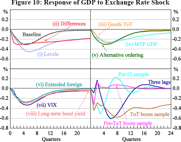
Figure 10 compares the response of aggregate GDP in our baseline model with the responses using alternative model specifications. The top two and bottom left panels contain eight alternative specifications:

1. GDP and the price level enter the VAR in log levels
2. GDP, the exchange rate and terms of trade enter in differences
3. The goods terms of trade replaces the goods and services terms of trade
4. The growth rate of Australia's major trading partners replaces US GDP growth
5. The exchange rate is ordered before the cash rate in the identification scheme
6. US CPI inflation and the US federal funds rate are included as additional foreign variables
7. The VIX index is included as an additional foreign variable
8. The Australian 10-year government bond yield is included as an additional domestic variable.

Compared to the baseline model, the levels specification implies a somewhat larger GDP response, while the peak effect in the differences specification is similar to the baseline model but occurs earlier. In both the levels and the differences specifications, the impact of an exchange rate appreciation is considerably more persistent. Although we prefer the specification with detrended GDP as it is more consistent with standard theoretical open economy models, VARs are often estimated with GDP in levels or differences specifications and these models suggest that our baseline results may understate the effect of exchange rate shocks on output.

In contrast, the model that includes US inflation and interest rates generates a path of GDP that is almost identical to our baseline model. This is reassuring as it suggests that the results in our baseline model adequately account for deviations from uncovered interest rate parity generated by changes in foreign monetary policy. The results are also largely unaffected by changing the measure of the terms of trade or the measure of foreign GDP that we include in the model, though in the latter case, the GDP response is somewhat more persistent. Allowing monetary policy to respond contemporaneously to the exchange rate shock makes little difference to our results, suggesting that we are not misidentifying monetary policy shocks as exchange rate shocks.

The response of GDP to an exchange rate shock in specifications including the VIX index and long-term bond yields are also nearly indistinguishable from our baseline results. The fact that including the VIX does not affect our results suggests that our identification scheme is not mistakenly capturing the effects of changes in investor risk premia rather than the effects of exchange rate movements. The fact that including long-term bond yields does not affect the results suggests that our identification strategy is not misinterpreting exchange rate movements caused by the expectation of future cash rate movements as exchange rate shocks.

The bottom-right panel of Figure 10 shows the responses of GDP to an exchange rate shock in a model including more lags as well as models estimated over alternative sub-samples. Although lag order selection tests favour two lags rather than three, a larger number of lags may allow the model to capture more completely the interactions between the responses of macroeconomic variables to exchange rate shocks. The response of GDP in the three-lag specification is roughly twice as large as that generated in our baseline results. The response of GDP also occurs later – it takes roughly a year for GDP to respond to the exchange rate shock. Once again, this could indicate that our model provides a lower bound to the effect of exchange rate shocks on output.

The three sub-samples that we consider are: a pre-inflation targeting sample (1985:Q1 to 1992:Q4); a pre-terms of trade boom sample (1993:Q1 to 2002:Q4) and a terms of trade boom sample (2003:Q1 to 2013:Q2). The point estimates from the pre-inflation targeting and terms of trade boom samples suggest a larger GDP response than our baseline results, while the middle sample points to a response that is similar in magnitude at its peak but shorter in duration. Although there is some evidence of sub-sample instability, this should be viewed in the context of the wide confidence bands around our baseline results.

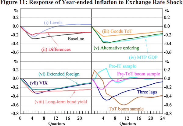
Figure 11 shows the response of year-ended inflation to an exchange rate shock in each of the model specifications discussed above. In general, the result from the baseline model is robust to changes in included variables and their ordering. In most models, the appreciation triggers a fall in year-ended inflation of between 0.2 and 0.4 percentage points five quarters after the shock, after which inflation gradually returns to trend.

As with the response of GDP to an exchange rate shock, the response of inflation is sensitive to the estimation sample. In the inflation-targeting era, an appreciation has a negative effect on inflation, though the estimated effect is noticeably larger and more persistent in the terms of trade boom sample. In contrast, inflation is estimated to rise following an exchange rate appreciation prior to the inflation-targeting era. Chung, Kohler and Lewis (2011) previously noted that the extent of exchange rate pass-through in Australia has varied over time.

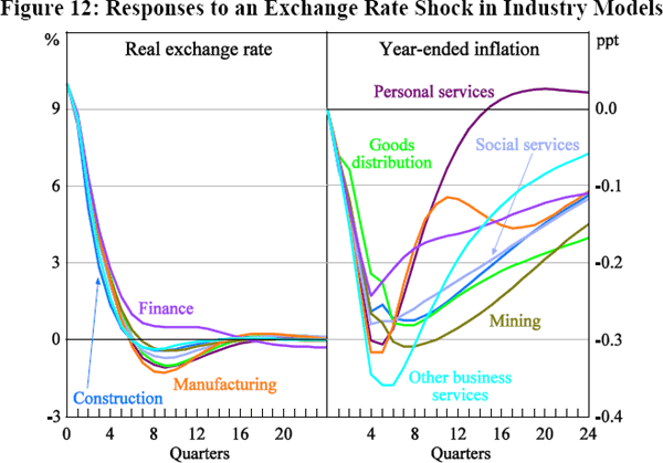
Because we estimate a separate VAR for each industry, one might be concerned that we do not identify the same exchange rate shocks for each industry. To examine whether this is the case, Figure 12 compares the responses of the exchange rate and inflation to an exchange rate shock in the various industry models. Reassuringly, the exchange rate response is almost identical across models. There is slightly more variation in the inflation response. However, in all models, the appreciation triggers a decrease in year-ended inflation of between 0.25 and 0.35 percentage points five quarters following the shock, after which inflation gradually returns to trend. On the basis of these results we are confident that the exchange rate shocks that we identify are similar across our industry models.^[20]

Footnote

We have also visually inspected the historical real exchange rate shocks implied by the industry models. They are virtually identical in all cases. [20]