RDP 2012-02: The Role of Credit Supply in the Australian Economy 4. Modelling the Role of Credit Frictions in the Australian Economy
May 2012 – ISSN 1320-7229 (Print), ISSN 1448-5109 (Online)
- Download the Paper 817KB
Our aim is to use an empirical method to assess the impact of credit frictions on the Australian economy and the extent to which shifts in credit supply explain historical variations in GDP and business credit.
We seek to identify the effects of credit supply shocks by using a structural VAR approach. This approach estimates the endogenous relationships between variables using a set of identification assumptions, so that exogenous (orthogonal) ‘shocks’ to the system can be recovered. The response of the system to these exogenous shocks – for example, a credit supply shock or monetary policy shock – can then be interpreted as revealing economic relationships free of endogeneity problems.
4.1 Structural VAR Technical Details
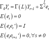
Technical details of the structural VAR approach are well-documented (Sims 1980; Hamilton 1994; Christiano, Eichenbaum and Evans 1999). We assume that the economy can be represented by the following structural form:
where:
- Yt is a n×1 vector of macroeconomic and policy variables.
- Γ0 is a non-singular matrix that captures the contemporaneous relationship between the variables, normalised to have 1's along the diagonal.
- Γ(L) is a matrix of pth order polynominals in the lag operator L, capturing the lag structure of the multivariate system.
-
et is a n×1 vector of serially uncorrelated,
orthogonal structural shocks, with
 being a diagonal matrix
of structural shock standard deviations.
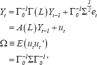
To identify the structural system, we must estimate a reduced-form VAR and impose sufficient restrictions to identify the structural parameters. The reduced form is:
Identification of the structural form involves recovering Γ0 and Σ from Ω. This requires sufficient restrictions
upon the form of Γ0 and Σ. Specifically, the
two matrices may have a total of no more than n(n+1)/2 unknown
parameters – the number of parameter estimates obtained from  . In addition, the restricted
Γ0 must be of full rank.
Typically, restrictions are ‘zero restrictions’ upon elements of Γ0 and Σ (keeping in mind that Σ is diagonal, and diagonal elements of Γ0 are normalised to 1). The simplest approach is to specify Γ0 as lower triangular – a Choleski ordering, or ‘recursive structure’. Under such a scheme, each variable in the ordering is predetermined with respect to subsequent variables in the ordering. Variables that are deemed more exogenous are placed higher in the ordering.
Recursive structures are usually difficult to justify on economic grounds and so non-recursive schemes whereby Γ0 is not lower triangular are often used (see Christiano et al (1999)). A non-recursive identification scheme is used in this paper.
4.2 Model Specification
Our structural VAR system consists of the following variables (for complete definitions see Appendix A):
- External sector. The external sector is captured by the log of Australia's major trading partner GDP (gdp*), the log of the RBA's Index of Commodity Prices deflated by the US GDP deflator (icp), a real foreign interest rate (r*) and the log of Australia's real trade-weighted exchange rate (rtwi).
- Domestic (non-credit) sector. The domestic (non-credit) sector is represented by the log of real gross national expenditure (gne), the log of real GDP (gdp), trimmed mean CPI inflation (π) and the cash rate (r). The latter three variables correspond with the three endogenous variables in the canonical New Keynesian DSGE model (Clarida, Galí and Gertler 1999). We follow Dungey and Pagan (2000, 2009) by including GNE in our model as well as GDP; as discussed in Dungey and Pagan (2000), GNE includes spending on imports and therefore it is likely that GNE and GDP react differently to variables such as the exchange rate.
These variables are generally consistent with other small open economy structural VARs, including Kim and Roubini's (2000) specification for advanced economies and previous Australian studies (e.g. Brischetto and Voss (1999); Dungey and Pagan (2000, 2009); Berkelmans (2005); Lawson and Rees (2008)). Finally, we also include:
- Domestic credit market. The Australian credit market is represented by the spread between the average variable lending rate paid by large businesses and the cash rate (spread), the log of aggregate real business credit (credit), and the ACCI-Westpac survey measure of difficulty obtaining finance (difficulty). In effect, these represent price, quantity and a measure of the tightness of supply for the business credit market.[18] In the baseline model we focus on the business credit market as this is most consistent with the use of the ACCI-Westpac survey variable.
As discussed, the difficulty variable is likely to have been affected by structural change in the economy over the past decade. Econometric tests identify a structural break in the mean of the series from September 2002.[19] Given that structural change in the manufacturing industry can be characterised as a gradual rather than sudden change, we account for the structural break in our baseline model by detrending the difficulty variable using a Hodrick-Prescott filter. In the robustness section we also consider two alternative possibilities: detrending the series using a deterministic trend from September 2002; and controlling for a mean shift from September 2002.
The logs of major trading partner GDP, Australian GNE, Australian GDP and business credit are detrended using a deterministic trend before entering the structural VAR model. The three foreign variables – gdp*, icp and r* – are treated as exogenous variables in the system. The system is estimated with two lags of both the endogenous and exogenous variables.[20]
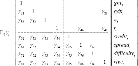
A non-recursive set of restrictions is placed on the contemporaneous relationships in our system. Each coefficient γij in the matrix Γ0 indicates that structural shocks to variable j affect variable i contemporaneously. The diagonal elements are normalised to 1, and blanks indicate elements that are constrained to equal zero.
The key aspects of our exactly identified scheme are explained below.
Credit market variables are assumed to react to real economy variables contemporaneously (the lower left quadrant of the matrix). The exception to this is that the spread is assumed not to react to inflation; that is, the nominal risk-free rate (r) can be thought of as comprising the real interest rate and compensation for (expected) inflation, with the additional spread on business loans compensating only for the additional risks involved in lending to businesses, such as credit and liquidity risk.[21] The difficulty-obtaining-finance variable and the credit spread are assumed to react contemporaneously to one another (γ67 and γ76), reflecting the possibility that banks adjust both the price and non-price terms of loans in accordance with their willingness to lend.
The central bank is assumed not to react to Australian GNE, GDP and inflation immediately, reflecting the lag with which these variables are observed. Monetary policy reacts immediately to movements in the credit spread (γ46), as this affects the rate paid by borrowers, but not directly to movements in the difficulty variable. That is, while policymakers might react quickly to the impact of a credit shock on loan pricing, they might wait for broader evidence of a change in lending standards rather than reacting immediately to the ACCI-Westpac survey variable. The central bank also takes into account contemporaneous information about the exchange rate when formulating policy (γ48).
Credit market variables are assumed not to affect output immediately. This might reflect the tendency for firms to use internal funds to maintain output in the short term, as well as lags between credit applications and settlement. Finally, the exchange rate is assumed to have a contemporaneous effect on GDP (through net exports), but a lagged effect on inflation.[22]
Footnotes
The set of credit market variables is somewhat analogous to the set of New Keynesian variables. Both sets contain a price and quantity term – inflation and output in the New Keynesian case, or spread and credit aggregate for the credit market. Also, both contain a ‘shifter’ variable that is the main focus – an aggregate demand shifter in the case of monetary policy, and a credit supply shifter in the case of the difficulty obtaining finance. [18]
A Bai-Perron test using a ‘mean + error’ specification indicated one structural break in the mean of the ACCI-Westpac series from September 2002 (this allowed for up to four regime changes, imposing a minimum regime length equivalent to 20 per cent of the sample). [19]
Akaike and Bayesian Information criteria for various model specifications suggest an optimal lag length of one, but an additional lag is included to absorb remaining serial correlation in some of the equations. [20]
The nominal business lending rate can be expressed as:
rb = r + s = (ρ
+ π) + s
View MathML
where: r is the nominal risk-free rate; s is the spread;
ρ is the real risk-free rate; and π is the inflation
premium, which compensates for expected inflation. This representation assumes
that the components are additive rather than multiplicative.
[21]
This is consistent with Chung, Kohler and Lewis (2011); their results indicate that the pass-through of exchange rate changes to overall consumer prices occurs gradually over an extended period. [22]


