RDP 2010-05: Direct Effects of Money on Aggregate Demand: Another Look at the Evidence 3. An Extended New Keynesian Model

In this section we discuss a model of the economy with an explicit equation describing the money market equilibrium. We use a standard closed-economy model with sticky-prices but extended by Nelson (2002) to include a cost to adjusting real money balances. This cost makes money demand forward-looking because it increases the incentives for households to smooth out their holdings of real money balances over time. There are three types of agents in the model: optimising households, profit maximising firms and a central bank that controls the settings of the nominal interest rate. The details are in Nelson (2002), so we just present the log-linearised equations that characterise the economy's equilibrium. Variables are expressed in log-deviations from steady state.

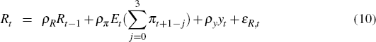
Equation (1) defines the log marginal utility of consumption, Ʌ_t, as a function of consumption, c_t, and a demand shock a_t. Equation (2) is the Euler equation linking the real interest rate, r_t, with the marginal utilities of consumption over time. Equation (3) defines the real interest rate as the difference between the nominal interest rate, R_t, and expected inflation, E_tπ_t+1. Equation (4) is the forward-looking Phillips curve implied by Calvo-price setting, where µ_t is the mark-up. Equation (5) comes from the labour market equilibrium condition, where n_t is hours worked and y_t is output. Equation (6) is the production function, where z_t is total factor productivity and k_t is the capital stock. Equation (7) is the goods market equilibrium condition. Equation (8) is law of motion of the capital stock, where x_t is investment.^[8] Equation (9) is the household's first-order condition for capital accumulation. Equation (10) is the monetary policy rule. Equations (11) and (12) are the exogenous processes followed by the demand shock and total factor productivity. Equation (13) is the demand for real money balances, m_t. Finally, ε_a,t, ε_m,t, ε_R,t and ε_z,t are identically and independently distributed (iid) type shocks with mean zero and standard deviations σ_a, σ_m, σ_R and σ_z.

Equations (1) to (13) govern the equilibrium dynamics of the 13 variables, a_t, c_t, R_t, k_t, n_t, x_t, r_t, y_t, z_t, Ʌ_t, π_t, m_t and μ_t. It might not be immediately apparent upon visual inspection of Equations (1) to (13) that money has no structural direct effects in this economy. But this is indeed the case, because the solution for all other variables is the same as the one that would obtain after having removed m_t and Equation (13) from the system. Put differently, money has no direct effects in this economy because m_t and Equation (13) are unnecessary to determine the equilibrium dynamics of the remaining 12 variables.

This, however, would not be the case if the central bank were to respond with the interest rate to movements in real money balances, so that real money balances enter the policy rule. In this case, it would be impossible to remove m_t and Equation (13) and still arrive at the same solution for the remaining variables. Money would have direct effects but in an artificially induced way. Real money balances would matter, but only because of the central bank's choice of incorporating them in the policy rule. The evolution of real money balances would then become relevant for households to forecast the path of the nominal interest rate; although, even in this case, money's additional influence would not be truly independent of the nominal interest rate.

The calibration, summarised in Table 5, is that of Nelson (2002). The parameters, g₁, g₂, g₃, g₄, κ₁, κ₂ and a_m are, in turn, functions of deeper structural parameters.

Table 5: Model Calibration

Parameter	Description	Value
g1	Function of structural parameters	15.41
g2	Function of structural parameters	−32.75
g3	Function of structural parameters	−15.53
g4	Function of structural parameters	3.58
β	Household's discount factor	0.992
αμ	Calvo price-setting parameter	0.086
α	Capital's share of income	0.36
sc	Consumption-to-output ratio in steady-state	0.72
δ	Depreciation rate	0.025
κ1	Function of structural parameters	0.046
κ2	Function of structural parameters	0.19
ρR	Coefficient on the lagged short-rate in the policy rule	0.29
ρπ	Coefficient on inflation in the policy rule	0.22
ρy	Coefficient on output in the policy rule	0.08
ρa	Persistence of demand shock	0.33
ρz	Persistence of technology shock	0.95
εm	Inverse of intertemporal elasticity of substitution in real money balances	5
am	Function of portfolio adjustment costs parameters	10
σa	Standard deviation of εa,t	0.01
σm	Standard deviation of εm,t	0.01
σR	Standard deviation of εR,t	0.002
σz	Standard deviation of εZ,t	0.007

The model can be written in matrix form and one of the available solution methods, like that of Uhlig (1995), can then be used to compute the rational expectations solution. If Y_t is the vector of jump variables, (y_t, Ʌ_t, r_t, n_t, x_t, μ_t)′, X_t is the vector of state variables, (a_t, k_t, z_t, c_t, R_t, π_t, π_t−1, m_t)′, and ε_t is the vector of iid shocks, (ε_a,t, ε_mt, ε_R,t, ε_z,t)′, then the unique solution is an equilibrium law of motion of the form:

where P, Q, R and S are the solution matrices.

One way to verify that money has no structural direct effects in this model is by rewriting the solution as a vector autoregression for the augmented vector . One would then notice that the coefficients on real money balances in the reduced-form equations for all variables other than real money balances are zero. In other words, for money to have direct effects, real money balances have to not only be a part of the state vector, X_t, as is the case here, but real money balances also have to matter for the rest of the system.

The solution expresses each endogenous variable as a linear combination of lags of the state variables and a linear combination of the structural shocks. In particular, the reduced-form equation for output, y_t, is the first row in Equation (15), which at the values shown in Table 5, is given by:

where is the reduced-form shock in the output equation, a linear combination of the structural shocks and is the first row of S. Note that real money balances do not enter Equation (16), so it's true coefficient is zero. And it is also the case that the money demand shock ε_m,t does not enter the reduced-form shock, .

Footnote

See Neiss and Nelson (2003). [8]